
Precision in irrigation design is rarely about simply placing water where it looks best on a plan. It is a strict exercise in physics. Whether you are designing a drip system for a high-density orchard or a sprinkler layout for open-field cultivation, small errors in your hydraulic calculations can lead to disastrous real-world results. A pressure variance that seems negligible in a spreadsheet can result in uneven crop growth, dry zones, or system failures due to water hammer.
For decades, agricultural engineers have relied on traditional spreadsheets to model these complex systems. While functional, these static sheets are often brittle. A single change in pipe diameter or a shift in topography often requires manually checking endless rows of cell references to ensure the logic holds. This "verification" mindset slows down the actual design process.
There is a more efficient way to handle these demands. By adopting a dynamic design workflow—specifically one that integrates Python directly into the spreadsheet grid—engineers can build models that update instantly and visibly. This guide covers how to set up a comprehensive irrigation model, from determining friction loss to analyzing uniformity metrics, using a modern approach that turns static data into real-time engineering insights.
The fundamentals of irrigation hydraulics
Before diving into the computational workflow, it is important to ground the discussion in the core physics that drive irrigation design. While a basic hydraulic calculation can be performed on paper for a single pipe, complex networks require a rigorous adherence to fluid mechanics principles to ensure the system performs as intended.
The first critical factor is friction loss. As water moves through a pipe, energy is lost due to the roughness of the pipe walls and the viscosity of the fluid. In irrigation, engineers typically rely on the Hazen-Williams equation or the Darcy-Weisbach equation to quantify this energy drop. Accurately modeling this is the only way to ensure that the pressure at the pump translates effectively to the pressure at the furthest emitter.
Velocity and the Reynolds number are equally important. Water must move fast enough to scour debris from the lines but slow enough to prevent dangerous pressure surges known as water hammer. Calculating the Reynolds number allows the designer to determine the flow regime—laminar, transitional, or turbulent—which directly impacts the friction factor used in head loss formulas.
Finally, the ultimate goal of these calculations is pressure uniformity. A well-designed system ensures that the first dripper in the row and the last dripper emit nearly identical amounts of water. If the hydraulic calculations fail to account for elevation changes or minor losses in fittings, uniformity drops, and the efficiency of the entire agricultural project is compromised.
Step-by-step: building the calculation workflow
Moving from theory to practice requires a tool that can handle iterative design. In a standard spreadsheet, this often looks like a "black box" of hidden formulas. In a tool like Quadratic, which combines spreadsheets with Python, the workflow becomes transparent and auditable. Here is how a user can structure a robust irrigation model.
Step 1: defining system parameters
The foundation of any hydraulic model is the input parameters. This includes the pipe roughness coefficient (C-factor), internal diameters, and required flow rates per emitter.
In a traditional setup, changing the C-factor to test a different pipe material might involve finding the specific cell that references it across multiple sheets. In a modern workflow, you can define these parameters as variables in Python. For example, setting a variable for the C-factor means that if you update it once, every calculation in the entire workbook re-runs instantly. This separates your raw data from your logic, reducing the risk of human error during data entry.
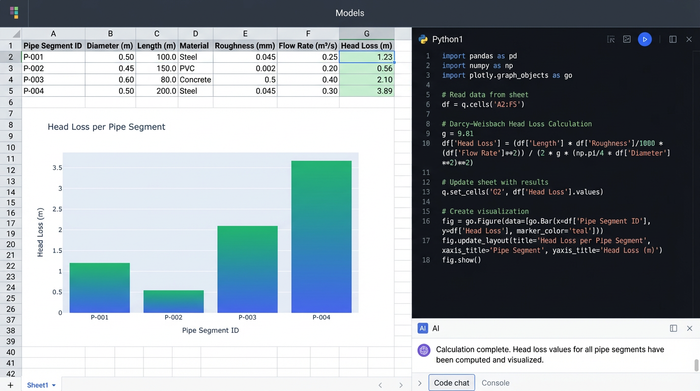
Step 2: calculating head loss
Calculating head loss is where standard spreadsheets often become messy. To determine the friction loss across pipe lengths and fittings, engineers often force complex mathematical logic into single-line formulas.
By using Python directly in the grid, you can script the logic for the Reynolds number and friction factors clearly. Instead of a nested Excel formula that is impossible to debug, you can write a short script that checks the velocity, calculates the Reynolds number, selects the appropriate friction factor, and outputs the head loss. This makes the math visible. If a peer reviews your work, they can read the code like a logical sentence rather than deciphering a string of cell references.
Step 3: determining pressure distribution
Once head loss is calculated, the next step is mapping the pressure at each node or dripper along the lateral. This involves subtracting the cumulative head loss and adjusting for elevation changes at every point in the system.
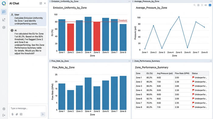
With the pressure mapped, you can calculate the Emission Uniformity (EU) metric. This is a standard efficiency indicator that compares the average emission of the lowest 25% of emitters to the average emission of the whole system. In a Python-enabled spreadsheet, you can automate this calculation to flag any zone where the EU drops below a set threshold, allowing you to catch efficiency problems immediately.
Visualizing the data: moving beyond static grids
One of the greatest risks in hydraulic design is the "visualization deficit." When an engineer stares at a grid containing 500 rows of pressure data, it is difficult to spot a specific zone where pressure dips below the allowable margin.
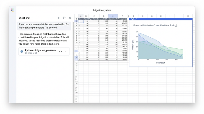
Modern tools allow you to bridge the gap between calculation and visualization. In Quadratic, you can generate a Pressure Distribution Curve directly next to your calculation data using Python plotting libraries. This graph visualizes the pressure profile along the length of the lateral line.
This creates a feedback loop. If the curve dips too low, the designer can adjust the pipe diameter in the input grid. Because the script and the graph are linked to the data, the hydraulic calculation updates, and the curve redraws itself instantly. This transforms the workflow from a static verification task into a dynamic design session, where you can visually "tune" the system for optimal performance.
Broader applications: mechanical vs. irrigation hydraulics
While this guide focuses on water distribution systems, the ability to script complex engineering math is valuable across the entire spectrum of fluid power and mechanics. The principles of fluid dynamics remain consistent, whether you are moving water through PVC pipes or oil through high-pressure steel lines.
Mechanical engineers, for instance, often rely on similar workflows when building a hydraulic cylinder force calculator. While the fluid and pressures differ, the need to calculate force based on pressure and area—while accounting for frictional losses—requires the same level of mathematical rigor. Similarly, sizing a power unit often involves a hydraulic horsepower calculator workflow to ensure the engine allows the pump to deliver the required flow at a specific pressure.
In both irrigation and heavy machinery, the variables change, but the need for custom logic remains. An engineer might need a hydraulic diameter calculation for non-circular ducts or a hydraulic radius calculator for open channel flow. In a standard spreadsheet, these specific formulas must be rebuilt manually every time. In a Python-integrated environment, these calculators can be saved as reusable functions, allowing engineers to build libraries of logic that apply to everything from a hydraulic hp calculator for a pump to a complex irrigation network.
Conclusion: from verification to design
The shift from static spreadsheets to dynamic, code-enabled tools represents a fundamental change in how engineers approach their work, facilitating advanced predictive modeling and analytics. It moves the focus from simply verifying that a design works to actively designing for optimization.
When your hydraulic calculations are visual, auditable, and automated, you spend less time checking cell references and more time refining the efficiency of the system. Whether you are calculating head loss for a drip line or evaluating the uniformity of a sprinkler zone, the tools you use should support the complexity of the physics, not hide it behind brittle formulas.
By adopting a workflow that integrates Python with familiar spreadsheet grids, irrigation designers can build models that are as resilient and efficient as the systems they aim to create. We invite you to try the irrigation hydraulics template in Quadratic, or explore the Python Intro Template, to experience the difference between static data entry and dynamic engineering design.
Use Quadratic for precise hydraulic calculations
- Automate complex hydraulic calculations: Replace brittle spreadsheet formulas with clear Python scripts directly in the grid for friction loss (Hazen-Williams, Darcy-Weisbach), Reynolds number, and other fluid dynamics.
- Build dynamic, auditable irrigation models: Define system parameters as Python variables so a single adjustment instantly updates all dependent calculations across your entire design.
- Visualize pressure distribution in real-time: Generate interactive pressure distribution curves alongside your data, allowing you to visually "tune" pipe diameters and instantly see the impact on your design.
- Ensure uniform water distribution: Automatically calculate Emission Uniformity (EU) to immediately flag zones where pressure drops below optimal thresholds, preventing uneven crop growth.
- Create reusable engineering functions: Build a library of custom hydraulic formulas and calculators in Python, making it easy to apply consistent logic across all your irrigation projects.
Ready to move from static verification to dynamic design? Try Quadratic.