Differential Equation Solver

Overview of the differential equation solver template

This python template provides a unified, single-sheet interface for numerical ODE integration, combining the computational power of Python with the interactivity of a spreadsheet. It allows users to define equations and tune parameters in a dedicated input section, eliminating the need to write full scripts from scratch to solve differential equations.

Key features include:

Integrated environment: Merges Python spreadsheet computation with standard spreadsheet cells.
Dedicated input: A specific section for defining equations and simulation parameters.
Visual feedback: Delivers immediate results via an automatically updating Plotly chart.
No setup required: Removes the friction of manual environment configuration.

Configuring simulation parameters

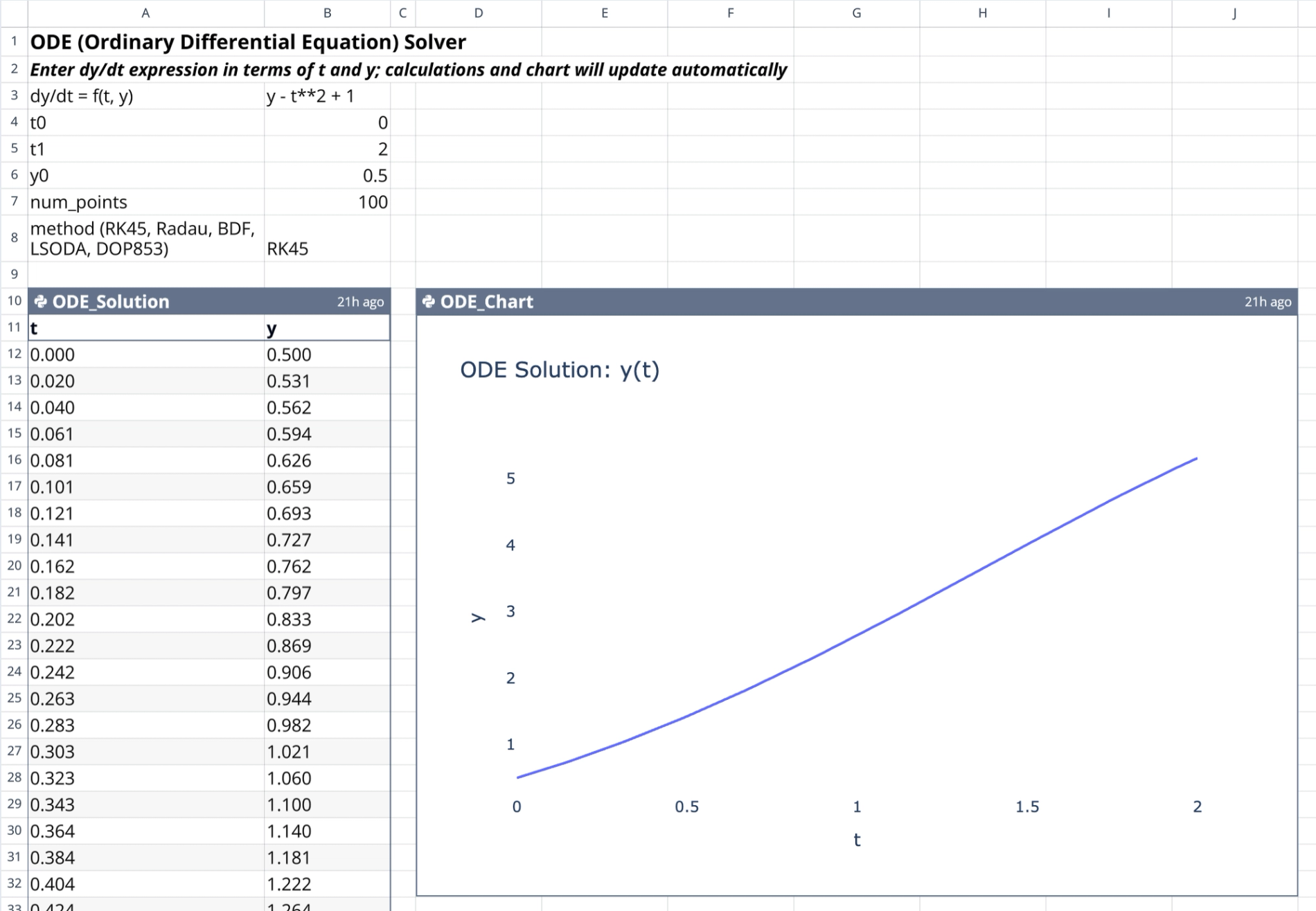
The input section (cells B3:B8) allows users to control the simulation without editing the underlying Python code.

Variable definition: The solver recognizes standard t (time) and y (state) variables for all expressions.
Equation entry: Users input the differential equation as a Python-evaluable string in cell B3 (e.g., "y - t**2 + 1").
Time boundaries: Cells B4 and B5 define the start (t0) and end (t1) points for the integration interval.
Initial conditions: Cell B6 establishes the starting value y0 at time t0.
Resolution control: Cell B7 determines the number of evaluation points, controlling the density of the output grid.
Method selection: Cell B8 offers a dropdown of Scipy solvers, including RK45, Radau, and LSODA, to handle various equation stiffness levels.

How the ODE differential equation solver works

The calculation engine

The core logic resides in the Python cell named ODE_Solution located at A10 in this coding spreadsheet. This cell handles the numerical integration process:

Library integration: It imports numpy, pandas, and scipy.integrate to handle mathematical operations and data formatting.
Data ingestion: The script reads parameters directly from the configuration range (B3:B8) using Quadratic’s cell referencing.
Safety parsing: User-provided strings are compiled within a restricted namespace containing only safe mathematical functions (like trigonometric and exponential functions) to prevent arbitrary code execution.
Numerical integration: The code executes solve_ivp to generate solution arrays based on the defined derivative function.
Data output: The results are formatted into a pandas DataFrame and returned to the grid, populating cells A10:B111.

The visualization engine

The visualization logic is contained in the ODE_Chart cell at D10.

Data source: This cell directly references the output table generated by the differential equation solver.
Plotting library: It utilizes Plotly Express to construct an interactive line chart, leveraging the power of python libraries for data visualization.
Layout: The chart plots the state variable y against time t, rendered with a clean white background for clarity.

Steps to solve differential equations

1. Input the desired differential equation string in the configuration section (Cell B3).

2. Adjust the time interval (t0, t1) and initial condition (y0) values to match the problem constraints.

3. Select the appropriate numerical method (e.g., RK45 for non-stiff, Radau for stiff problems).

4. Observe the ODE_Solution table automatically populating with calculated data points.

5. View the ODE_Chart to analyze the trajectory and behavior of the solution.

6. Modify any input value to instantly trigger the reactive calculation chain and update the visualization.

Who this Differential Equation Solver is for

Engineering students who need to verify homework solutions or visualize dynamic systems without setting up complex environments.
Researchers requiring a rapid interface to identify the differential equation solved by specific parameter sets.
Data scientists looking to prototype ODE models quickly before deploying them in larger applications.
Educators demonstrating the behavior of differential equations and the impact of initial conditions in real-time.

Use Quadratic to solve differential equations with dynamic charts & solutions

Define differential equations and simulation parameters directly in spreadsheet cells.
Visualize solutions instantly with interactive, automatically updating Plotly charts.
Select from multiple Scipy solvers (RK45, Radau, LSODA) to match equation stiffness.
Adjust time intervals, initial conditions, and resolution to explore scenarios in real-time.
Perform robust numerical integration with Python libraries, without writing full scripts.
Receive structured solution data output directly into the grid for further analysis.

Duplicate this Differential Equation Solver file