Template overview
This Python template demonstrates a functional radioactive decay calculator within a single sheet. It models exponential decay using customizable input parameters and visualizes the relationship between half-life and remaining quantity over time. By leveraging Quadratic’s reactive execution, the template updates data and charts instantly whenever inputs change.
Input parameters and configuration
The left portion of the sheet (Columns A and B) contains the configuration settings. Labels and units are organized in Column A for clarity, while Column B holds the editable numeric values.
- Primary inputs (Column B):
- Initial amount ($N_0$): The starting quantity of the substance (default is 100).
- Half-life ($t_{1/2}$): The time required for the quantity to reduce by half.
- Total time: The full duration of the simulation.
- Time step: The interval size for calculation increments.
- Calculated constants:
- Decay constant ($\lambda$): Automatically computed in cell B8 using the formula $LN(2) / \text{half-life}$.
- Specific time evaluation: Calculates the remaining amount for a single specific time point ($t$).
- Structure: This section serves as a transparent radioactive decay formula calculator, allowing users to see exactly how constants are derived before they are passed to Python.
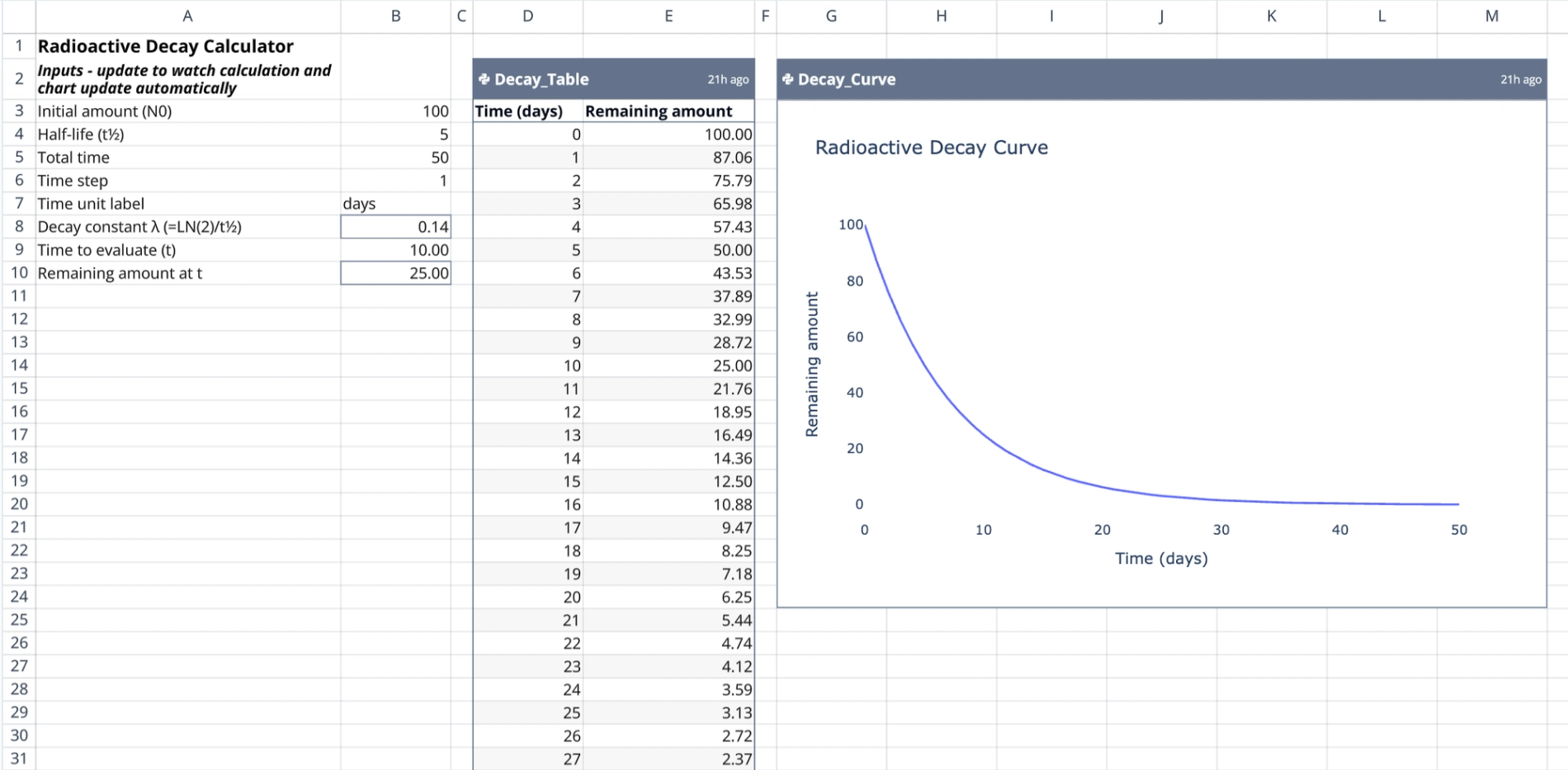
Generating the data table via Python
A Python script anchored in cell D2 generates the core data for the model. This script imports the input values from Column B and constructs a two-column DataFrame named Decay_Table.
- Calculation logic: The script iterates through time steps from 0 to the defined total time. It applies the standard exponential decay formula: $N(t) = N_0 \times (1/2)^{(t/t_{1/2})}$.
- Output range: The resulting table spans cells D2:E54.
- Column 1: Lists time increments based on the defined time step.
- Column 2: Lists the calculated remaining amounts, providing a step-by-step radioactive decay calculation example.
Visualizing the decay curve
A second Python script, anchored at cell G2, generates the visualization for the model. This script references the Decay_Table data frame directly to ensure the chart and data remain synchronized.
- Chart features: The chart is named
Decay_Curveand spans the range G2:M24. - Plotting: It plots time on the x-axis and the remaining amount on the y-axis, visually representing the asymptotic approach to zero as the radioactive material decays.
Interacting with the template
The template is designed for dynamic exploration. Users can modify variables in Column B, such as changing the half-life from 5 to 10 or adjusting the initial amount.
- Reactive updates: When an input changes, the Python cells at D2 and G2 automatically re-execute. The data table and decay curve regenerate instantly to reflect the new parameters.
- Use cases:
- Simulating the decay rates of different isotopes.
- Acting as a flexible online radioactive decay calculator for educational demonstrations.
- Testing various time steps to adjust the granularity of the data.
Who this Radioactive Decay Calculator is for
- Educators: Teachers demonstrating the mathematical concepts of half-life and exponential functions.
- Students: Learners needing a radioactive decay half life calculator for physics or chemistry coursework.
- Researchers: Scientists requiring a quick radioactive decay model calculator for estimations.
- Quadratic Users: Developers exploring how to chain spreadsheet inputs, Python logic, and visualizations into a cohesive tool.
Use Quadratic to calculate radioactive decay
- Customize initial amount, half-life, total time, and time steps directly in the spreadsheet.
- See calculated constants and decay formulas transparently before Python execution.
- Generate precise decay data tables using embedded Python scripts.
- Visualize the decay curve instantly with synchronized charts that update reactively.
- Dynamically simulate decay rates for different isotopes and adjust data granularity.