Financial valuation: build a multi-method model

Financial valuation sits at the intersection of art and science. It requires the rigorous application of mathematical formulas alongside the nuanced judgment of market conditions. However, for years, the tools available to finance professionals have forced a compromise between speed and depth.

In a traditional workflow, an analyst opens a spreadsheet, creates a tab for data entry, a tab for the Discounted Cash Flow (DCF) model, and a separate tab for comparable company analysis (Multiples). Inputs like the risk-free rate or current share prices are often hard-coded—typed in manually from a separate browser window. The moment that data is entered, it is stale. Furthermore, comparing the outputs of absolute and relative valuation methods usually requires flipping between tabs or building a static summary sheet that breaks as soon as a row is added.

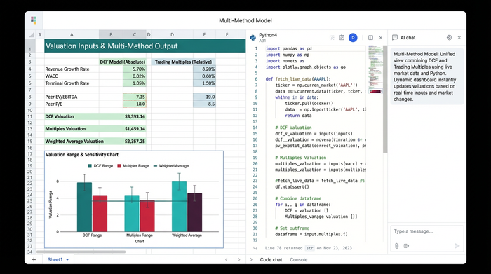
To make better investment decisions, we need a "Multi-Method Model." This approach performs financial valuation using both absolute and relative methods simultaneously, powered by live data rather than static inputs. By utilizing Quadratic’s infinite canvas and native Python integration, you can build a model that unifies these disparate workflows into a single, dynamic dashboard.

The core approaches to financial valuation

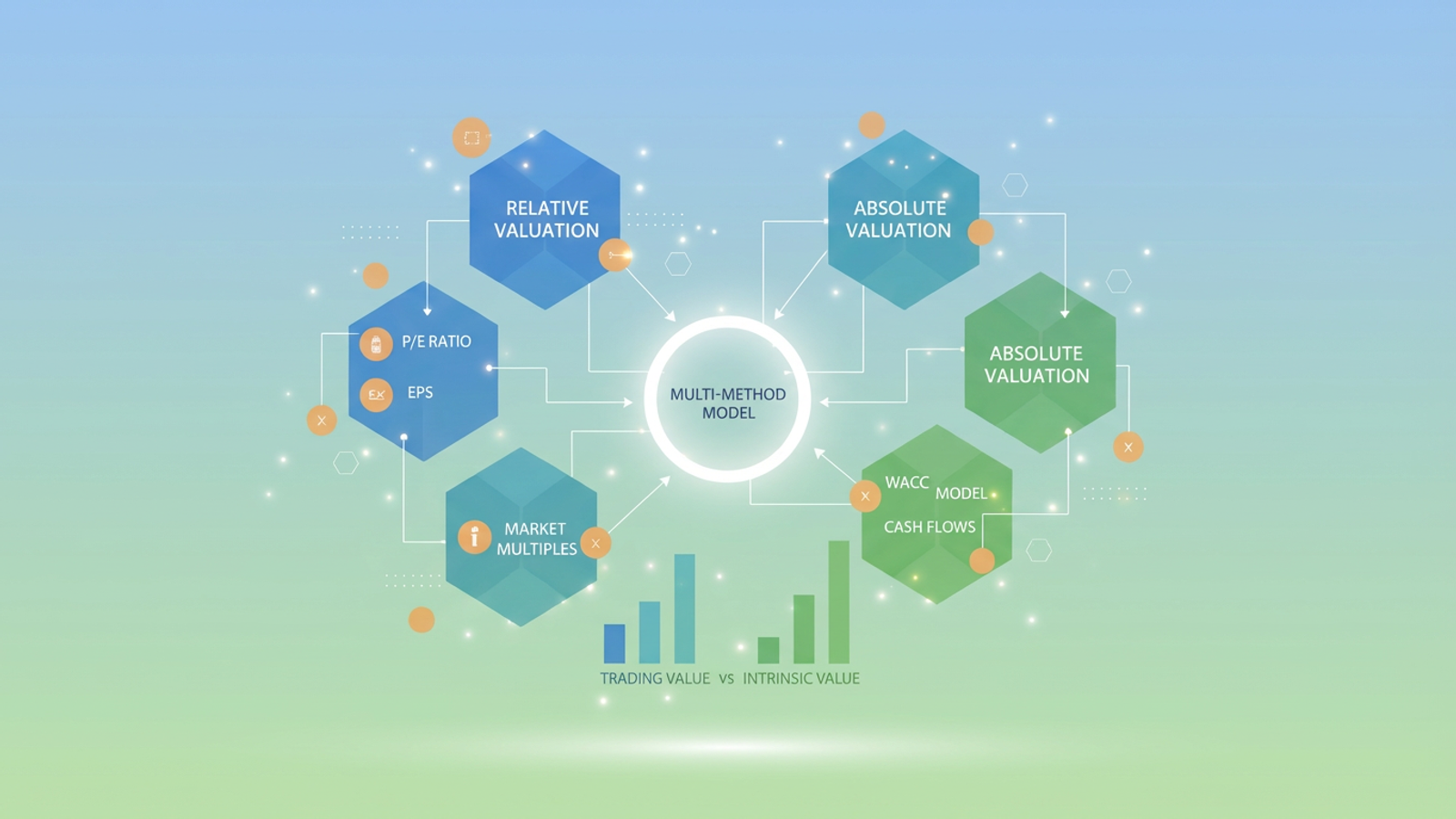
Before diving into the construction of the model, it is helpful to distinguish the two primary schools of thought that we will be integrating. Most financial modeling and financial analysis coursework treats these as distinct exercises, but in practice, they must inform one another.

Relative valuation involves comparing a company’s value to its peers. This relies on metrics like Price-to-Earnings (P/E) ratios, Earnings Per Share (EPS), and Enterprise Value multiples. It answers the question: "How much is the market paying for a dollar of earnings in this sector?"

Absolute valuation, conversely, attempts to determine the intrinsic value of an asset based on its projected future cash flows, discounted back to the present. This includes methods like the Dividend Discount Model (DDM) or the standard DCF.

While academic courses on financial statement analysis and valuation often teach these methods in isolation, modern decision-making requires a holistic view. A discrepancy between a company’s intrinsic value (Absolute) and its trading value (Relative) is often where the investment opportunity—or the risk—lies. In this guide, we will build a model that calculates both simultaneously.

Step 1: Automating market inputs (the dynamic data advantage)

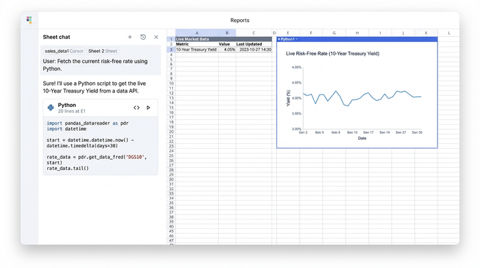
The greatest weakness in traditional valuation financial modeling is static data. If you are building a model today, you likely open a financial news site, look up the 10-year Treasury yield for your risk-free rate, and type "4.2%" into a cell. Next week, you have to remember to update it.

In Quadratic, we replace manual entry with Python. Because Quadratic allows you to write Python directly in the spreadsheet cells, you can pull live market data via APIs or libraries like yfinance without needing complex plugins.

For this use case, we need several key market inputs to drive our formulas:

• Current share price
• Historical dividends
• Equity Beta
• Risk-free rate
• Market return

Instead of hard-coding the Equity Beta, you can write a short Python script in a cell to fetch the stock’s historical volatility against the market index and calculate Beta automatically. Similarly, the risk-free rate and share price can be pulled live. This ensures that every time you open your model, your baseline assumptions reflect the current reality of the market, not the reality of last Tuesday.

Step 2: Building the relative valuation engine

With our live data flowing into the canvas, we can construct the relative valuation section. On a standard spreadsheet, this might be buried in "Sheet 2." On an infinite canvas, we can place this logic directly to the right of our data source, keeping the lineage of the data visible.

To build the relative valuation engine, we focus on the "Multiples" aspect of the workflow. First, we calculate the EPS value per share and Distributable earnings based on the company's latest financial statements. Using the live share price we pulled in Step 1, we can instantly compute the current P/E ratio.

From here, we can derive the Total Equity Value via Earnings. By setting this up as a formula that references our live Python cells, we create a dynamic output. If the share price shifts or if we adjust our earnings assumptions, the implied valuation updates instantly. This section serves as our market sentiment anchor—telling us what the market currently believes the company is worth.

Step 3: Constructing the absolute valuation model

Next, we move to the absolute valuation. This is generally the most technical part of the workflow for a financial modeling & valuation analyst, as it requires building a bridge between market risk and projected company performance.

Calculating the cost of capital

To discount future cash flows, we need a discount rate, typically the Weighted Average Cost of Capital (WACC). In a traditional sheet, this is often a "black box" calculation. In Quadratic, we make it transparent.

Using the live Equity Beta, Risk-free rate, and Market return established in Step 1, we calculate the Cost of Equity using the Capital Asset Pricing Model (CAPM). If the company has debt, we would also factor in the cost of debt and the corporate tax rate to arrive at the final WACC. Because the Beta is live, your discount rate automatically adjusts to changes in the stock's volatility profile.

The dividend discount and DCF logic

With the discount rate established, we project the cash flows. For a dividend-paying stock, we might use a Dividend Discount Model. We forecast the Next year dividend value per share by applying a Dividend growth rate to the historical dividend data.

We then calculate the Total Equity Value via Dividend Method. However, real-world financial statement analysis and security valuation are rarely this simple. We must often account for one-off items. In this use case, we add the Present value of synergy benefits (perhaps from a recent merger) and the Net proceeds from asset disposal, while subtracting the impact of Corporate tax.

Aggregating these figures gives us the Total DCF Value. This number represents the intrinsic value of the company based on its fundamentals, independent of its current stock price.

Step 4: Visualizing the valuation for stakeholders

The final step is presentation. A grid of numbers is rarely enough to persuade a CFO or an investment committee. This is where the infinite canvas becomes a powerful differentiator for a financial advisor practice valuation calculator or an internal corporate presentation.

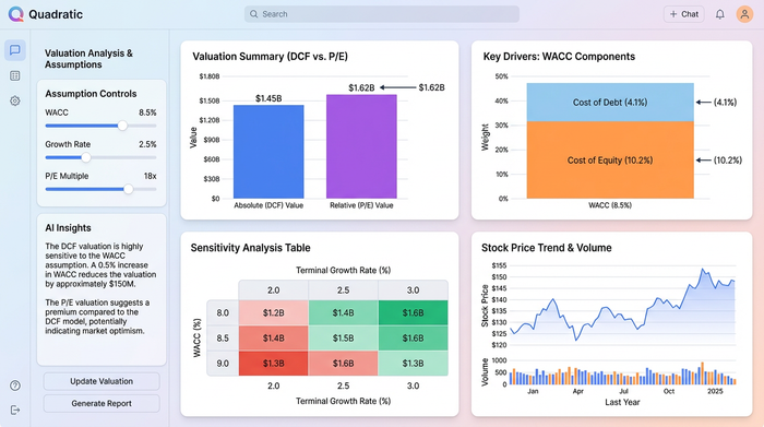
Because we are not restricted by grid boundaries, we can place the Relative Valuation results (Step 2) and the Absolute Valuation results (Step 3) side-by-side. We can then use Quadratic’s charting features to visualize the spread between the two.

Imagine a sensitivity table that is not just a static block of text, but an interactive element. You can create a dashboard where stakeholders can adjust the Dividend growth rate or the Synergy benefits assumptions, and immediately see how those changes impact both the P/E implied value and the DCF value on a comparative bar chart. This turns the model from a static artifact into a conversation piece, allowing for real-time scenario planning during meetings.

Bridging theory and practice

Certifications like the financial modeling & valuation analyst FMVA certification provide an excellent foundation in the theory of these models. They teach the formulas, the accounting principles, and the logic behind discounting cash flows. However, the execution of these concepts has historically been limited by the tools available.

Moving from a static spreadsheet to a dynamic, code-enabled environment bridges the gap between theory and modern data science. It allows analysts to apply the rigorous theoretical frameworks they have learned while eliminating the manual drudgery and error-prone data entry that often plagues the actual work.

Conclusion: The future of financial modeling

By leveraging Quadratic, we have transformed a standard valuation exercise into a robust, automated workflow. We replaced hard-coded market inputs with Python scripts that pull live data. We moved from siloed tabs to a unified infinite canvas that displays Relative and Absolute valuations side-by-side. Finally, we turned static outputs into interactive visualizations that support better decision-making.

The future of financial valuation is not about choosing between complexity and speed; it is about integrating them. We encourage you to stop building models that go stale the moment they are saved and start building dynamic, multi-method models that evolve with the market.

Try building this valuation workflow in Quadratic today and experience the difference of a truly modern financial modeling platform.

Use Quadratic to build dynamic multi-method financial valuation models

• Automate market inputs: Pull live market data (e.g., risk-free rate, share price, beta) directly into your model using native Python, replacing manual entry and ensuring real-time accuracy.
• Unify valuation methods: Integrate absolute (DCF, DDM) and relative (multiples) valuation on a single infinite canvas for a holistic view, eliminating the need for separate, disconnected tabs.
• Ensure transparent calculations: Build and display the logic for complex calculations like WACC and CAPM transparently within the sheet, dynamically adjusting with live market data.
• Visualize comparative insights: Present absolute and relative valuation results side-by-side with interactive charts and dashboards, enabling real-time scenario planning and clear stakeholder communication.
• Eliminate stale data: Your model updates automatically with market changes, removing manual drudgery and ensuring your valuation assumptions are always current.

Ready to build more robust and dynamic valuation models? Try Quadratic.