
Last mile delivery logistics is widely recognized as the most expensive and complex segment of the supply chain, often accounting for up to 53% of total shipping costs. For operations managers and analysts, the pressure to reduce these costs is immense, but the barrier to optimization is rarely a lack of effort—it is usually a lack of data visibility. Most logistics teams sit on mountains of raw trip data, including timestamps, location codes, and driver logs. However, turning this raw information into actionable insights is difficult because the data is often too messy for standard spreadsheets yet too fluid for rigid enterprise dashboards.
The core issue lies in how trip data is recorded. A single delivery isn't a single row of data; it is a collection of status updates, GPS pings, and zone changes. To understand performance, analysts must perform "Trip Characteristics Analysis"—a method of reshaping data to view the full lifecycle of a shipment. This article explores how to bridge the gap between basic spreadsheet formulas and complex database queries using Quadratic. By mastering this workflow, you can move beyond simple averages and uncover the granular details that drive efficiency in last mile delivery logistics.
The data challenge in last mile delivery logistics
Managing data for final-mile operations is uniquely difficult because of the sheer volume of variables involved. This complexity scales rapidly. For example, the challenges scaling 4pl last-mile delivery health logistics involve intricate coordination between multiple stakeholders in difficult geographic environments. While the specific geography changes, the data problem remains the same: you need granular visibility into every movement to ensure reliability.
In a typical raw dataset, the structure of trip data is often "many-to-one." This means a single Shipment ID appears in multiple rows. You might have one row for the pickup scan, several rows for in-transit updates, and a final row for the drop-off. Each row contains a timestamp, a zone, and often a static value for the total distance of the trip.
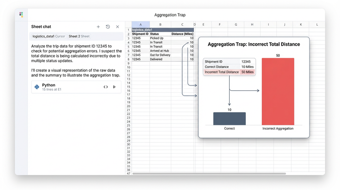
This structure creates what is known as the "Aggregation Trap." This is a specific analytical failure that occurs when analysts use standard pivot tables to summarize data. If you group your data by Shipment ID in a standard spreadsheet, the software may default to summing the distance column. If a 10-mile trip generates five status update rows, a standard summation will report that the driver traveled 50 miles. This inflation of distance data skews cost calculations, distorts driver performance metrics, and renders the analysis useless for legitimate last mile delivery logistics solutions.
Step-by-step: Analyzing trip characteristics in Quadratic
To solve the aggregation trap and get a true picture of performance, you need to flatten the data. The goal is to create a summary table where each Shipment ID appears exactly once, containing the start time, end time, origin zone, destination zone, and the correct distance.
Here is how you can perform this analysis using Quadratic, bridging the gap between manual Excel work and SQL queries.
1. Ingesting the raw data
The process begins by bringing your raw dataset into Quadratic. This data likely comes from a Transportation Management System (TMS) or a carrier CSV export. It will include columns for Shipment ID, Timestamp, Zone, Status, and Distance. Because Quadratic functions as a modern spreadsheet, you can view and manipulate this data in a familiar grid interface, but with the added ability to handle larger datasets without performance lag.
2. Grouping by shipment ID
To analyze the trip, you need to define the start and end of the journey. Since the data is spread across multiple rows, you cannot simply look at a single cell. You need to group the data by Shipment ID and apply logic to extract the correct timestamps.
- Pickup Time: You do not want an average time; you need the earliest timestamp associated with that ID. In data terms, this is the MIN value.
- Dropoff Time: Conversely, the completion of the delivery is the latest timestamp, or the MAX value.
- Zones: To understand the route, you need to extract the Zone associated with the MIN time (the Origin) and the Zone associated with the MAX time (the Destination).
3. Solving the distance problem
This is where the differentiation of using a tool like Quadratic becomes critical. To avoid the aggregation trap described earlier, you must handle the distance column differently than the timestamp columns.
In a standard pivot table, you have limited options for aggregation. In Quadratic, you can use SQL or Python directly in the sheet to specify exactly which value you want. Instead of summing the distance column, you can select the FIRST, UNIQUE, or MAX value for that column.
If a shipment has five rows and every row lists the distance as "10 miles," asking for the MAX value will return "10." Asking for the SUM would return "50." By selecting the correct aggregation method, you ensure that your summary table reflects the physical reality of the route, regardless of how many digital status updates were generated during the trip.
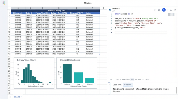
4. Visualizing the result
Once the logic is applied, the output is a clean, flattened table. You now have a dataset where every row represents a completed delivery. You can easily calculate the "Time to Delivery" by subtracting the Pickup Time from the Dropoff Time, and you can trust that the distance column is accurate. This clean dataset is now ready for visualization or export to finance teams for reconciliation.
Why Python/SQL integration matters for logistics
The logistics industry is currently seeing a shift in the tools used for analysis. Many of the top logistics data analytics solutions for last-mile delivery optimization are moving away from rigid spreadsheets because they cannot handle the logic required to clean "messy" data efficiently. However, moving entirely to a code-based workflow is often too technical for operations planners.
Quadratic offers a middle ground. It allows analysts to write SQL queries directly within the spreadsheet grid. You can write a query using GROUP BY Shipment_ID to perform the complex aggregations described above without needing to set up a separate database or request support from an IT department. This approach provides the reproducibility and speed of code while maintaining the visibility and ease of use of a spreadsheet. If you need to audit a specific shipment, the data is right there in the grid, not hidden behind a script.
Strategic benefits of accurate trip analysis
Moving from raw dumps to a clean "Trip Characteristics" table unlocks several strategic benefits for last mile delivery in logistics.
Operational efficiency
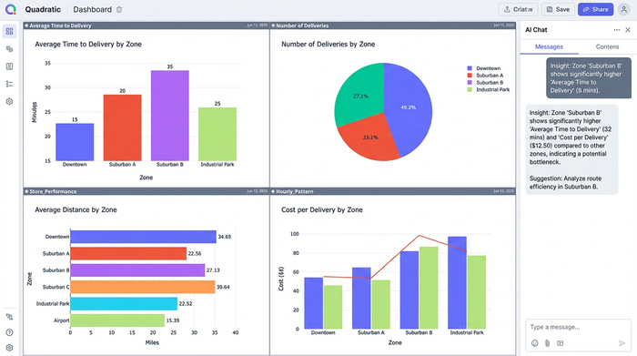
By accurately measuring the duration between the earliest and latest timestamps, you get a true "Time to Delivery metric". You can aggregate these times by Zone to identify which neighborhoods or regions are causing delays. If specific zones consistently show high durations despite short distances, you may have identified a bottleneck related to parking, traffic, or access codes.
Cost control
Logistics last mile delivery costs are often calculated based on mileage. If your data analysis accidentally inflates mileage due to the aggregation trap, you cannot effectively audit 3PL invoices or driver pay. Accurate distance data ensures you are paying for the work performed, not the number of rows in a database.
Competitive intelligence
With clean data, you can benchmark your own performance against industry standards. If you have access to external market data, you can even begin analyzing cdl last mile competitors logistics delivery performance to see where your network outperforms or lags behind the competition.
Conclusion
Effective analysis in last mile delivery logistic operations requires more than just summarizing columns. It requires a fundamental reshaping of data to reflect the real-world lifecycle of a shipment. Relying on basic averages or standard pivot tables can lead to the aggregation trap, where distance and costs are grossly overestimated.
By using a tool that handles data reshaping flexibly, analysts can turn messy driver logs into clear strategic insights. Quadratic provides the necessary environment to mix SQL precision with spreadsheet visibility, ensuring that your data tells the true story of your supply chain. For your next trip analysis project, consider using a workflow that allows for granular grouping and accurate aggregation to streamline your operations.
Use Quadratic to optimize last mile delivery logistics
- Transform raw trip data: Convert messy, multi-row logistics data into clean, single-entry summaries for each shipment.
- Avoid the aggregation trap: Accurately calculate trip distances and durations using precise aggregations (MIN, MAX, UNIQUE) to prevent inflated metrics.
- Extract key trip characteristics: Easily determine true pickup times, drop-off times, origin, destination, and correct distances for every delivery.
- Uncover operational insights: Identify bottlenecks, optimize routes, and gain granular visibility into driver performance and zone efficiency.
- Control costs with confidence: Ensure accurate mileage and time data for auditing 3PL invoices and driver pay.
- Combine spreadsheet familiarity with code power: Apply SQL and Python logic directly in a familiar grid, making complex analysis accessible without leaving your sheet.
Ready to optimize your last mile operations with accurate data? Try Quadratic.