Asset acquisition: build a robust financial model in excel (and beyond)

Strategic growth often hinges on the ability to identify and secure the right resources at the right price. Whether you are analyzing a headline-grabbing deal like the T-Mobile UScellular assets acquisition approval or evaluating the portfolio moves of a specialized entity like Real Asset Acquisition Corp, the fundamental challenge remains the same: financial valuation.

For financial analysts and corporate development professionals, the asset acquisition model is the tool of choice for determining whether a deal will be accretive or dilutive. However, while the strategy behind buying assets is sound, the modeling process is often fraught with risk. Traditional Excel models for asset acquisition frequently become fragile "black boxes." They are difficult to audit, prone to broken reference errors when rows are added, and cumbersome to update when testing dynamic operational scenarios.

To make confident investment decisions, analysts need a modern financial model—one that combines the familiar grid interface of spreadsheets with the transparency and computational power of Python. By moving your workflow into Quadratic, you can build asset acquisition models where the logic is visible, the data is dynamic, and the path to Net Present Value (NPV) and Internal Rate of Return (IRR) is clear and auditable.

Understanding the basics: asset acquisition vs. business combination

Before a single cell is populated in your model, the deal structure must be clearly defined. The distinction between accounting for asset acquisitions versus business combinations is not merely semantic; it dictates the tax implications, liability assumptions, and the very inputs that drive your financial model.

In an asset acquisition, the buyer purchases specific assets—such as inventory, equipment, intellectual property, or client lists—without necessarily assuming the seller's liabilities. This allows the buyer to "cherry-pick" what they need. In contrast, a business combination (often a stock deal) involves acquiring the entity itself, meaning the buyer inherits the target's legal and financial history, including debts and potential lawsuits.

When modeling, the keyword here is purchase price allocation. In an asset deal, the purchase price is allocated to individual assets, which resets their basis for depreciation. This step is critical because it directly impacts the tax shield and, consequently, the free cash flow. This allocation is formally reported on the Instructions for Form 8594 asset acquisition statement filed with the IRS. Your model must accurately reflect these allocations to project future tax liabilities correctly.

In a traditional spreadsheet, toggling between the tax logic of an asset acquisition vs. business combination often requires complex, nested IF statements that are prone to breaking. In Quadratic, you can handle this elegance using Python. You can set "Deal Type" as a variable in your code. With a simple conditional statement, the model can automatically switch depreciation schedules and tax logic across the entire analysis, ensuring your outputs align with the specific structure of the deal without cluttering your grid with fragile formulas.

Step 1: structuring your model inputs

A robust financial model separates assumptions from calculations. When dealing with complex valuations, scattering hard-coded numbers across multiple sheets makes the model impossible to audit. Instead, you should centralize your inputs to drive the logic downstream.

For a comprehensive asset acquisition model, you will need to aggregate data across three primary categories:

1. Capital costs: This includes the purchase price of the assets, transaction fees, and estimated residual values at the end of the useful life.

2. Operational inputs: These are the drivers of the asset's performance, such as useful life, unit pricing, production capacity, and usage metrics.

3. Economic factors: External variables like the corporate tax rate, inflation assumptions, and the discount rate (WACC).

Different industries will require highly specific input fields. For example, if you are modeling based on clinical stage pharmaceutical assets acquisition criteria, your inputs might include probability-adjusted R&D milestones, patent expiration dates, and FDA approval timelines.

In standard spreadsheets, these inputs often live on a static "Inputs" tab. If you need to pull in historical data to justify an assumption, you have to copy-paste it manually. Quadratic improves this workflow by allowing you to query data directly using SQL or Python, a key aspect of effective financial data analytics. You can keep your inputs in a clean, centralized data frame that feeds the entire model. If market conditions change, you update the data source, and the model recalculates instantly without manual intervention.

Step 2: modeling operational scenarios (cost & revenue)

Once the inputs are set, the next step is to model the operational reality of the assets. This involves projecting revenue and calculating the cost function. A sophisticated model must distinguish between fixed costs (which remain constant regardless of output) and variable costs (which scale with production).

In a traditional spreadsheet, modeling a 10-year financial forecast often involves dragging a formula across hundreds of columns or down thousands of rows. If the logic changes—for instance, if variable costs need to scale non-linearly after a certain production threshold—you have to rewrite the formula and re-drag it, risking copy-paste errors.

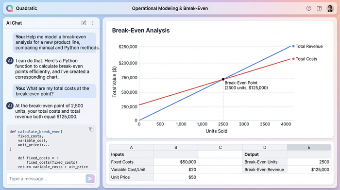
Quadratic allows you to define these relationships using Python functions. You can write a simple function for total_cost that takes fixed costs, variable costs, and quantity as arguments. You can then apply this function to your entire dataset in one step. This approach not only saves time but also makes the logic transparent. Anyone reviewing the model can read the code to understand exactly how costs are derived.

This flexibility is particularly useful for break-even analysis. By automating the calculation of the critical production quantity—the point where revenue covers both fixed and variable costs—you can instantly see how changes in unit pricing or efficiency impact the viability of the acquisition. You can solve for the break-even point mathematically in Python, providing a precise figure rather than an approximation derived from a data table.

Step 3: investment appraisal & financial metrics

The core of any acquisition model is the investment appraisal. This is where you determine if the deal makes financial sense. The model must calculate the cash flows generated by the assets and discount them back to the present day.

Your calculations should flow logically:

1. Depreciation: Calculate the depreciation expense based on the allocated purchase price (referencing the logic needed for the Form 8594 asset acquisition statement). This figure is crucial for calculating the tax shield.

2. Imputed interest & total costs: If the acquisition is financed, calculate the interest expense to arrive at the total cost of ownership.

3. Profitability: As part of your P&L analysis, deduct costs from revenue to find Gross and Net Profit.

Once the cash flows are projected, you move to the dynamic metrics: Net Present Value (NPV) and Internal Rate of Return (IRR).

• Net Present Value (NPV): This metric tells you the value of the projected cash flows in today's dollars, accounting for the risk profile of the investment. A positive NPV generally signals a go decision.
• Internal Rate of Return (IRR) & Payback Period: These metrics measure the efficiency of the investment and how quickly the initial capital outlay will be recovered.

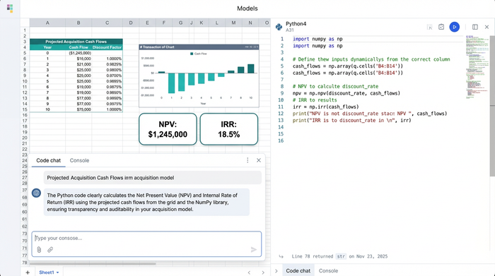
In traditional Excel, these calculations are often hidden inside opaque cell references like =NPV(C4, D10:D50). An auditor cannot see what C4 represents without tracing precedents. In Quadratic, you can use a Python library like NumPy to perform these calculations explicitly. A line of code reading np.npv(discount_rate, cash_flows) is self-documenting. It tells the reviewer exactly what is happening, ensuring that the financial logic is sound and the results are trustworthy.

Step 4: visualizing scenarios on the infinite canvas

Valuation is rarely about a single number; it is about a range of possibilities. Analysts typically need to compare a Base Case, an Optimistic Case, and a Pessimistic Case. In standard spreadsheets, this usually requires duplicating tabs or building complex data tables that make the file heavy and slow.

Quadratic changes this paradigm with the Infinite Canvas. Because the workspace is not limited to a standard grid, you can place the "Acquisition A" model directly next to "Acquisition B" on the same view. You are not forced to toggle between tabs to compare outcomes.

Furthermore, you can use Python visualization libraries like Plotly or Matplotlib to create dynamic graphs that sit right next to your data. Imagine a break-even chart where the revenue curve intersects the cost curve. In Quadratic, as you tweak the "Purchase Price" or "Interest Rate" variables, the intersection point on the graph updates instantly. This allows for real-time sensitivity analysis during meetings, where stakeholders can visually see how changes in assumptions impact the profit curve and investment viability.

Best practices for auditing your asset acquisition model

The difference between a good model and a great one often comes down to auditability, aligning with established financial modeling best practices. Asset acquisition modeling requires precision; a mistake in a depreciation formula or a broken cell reference can skew the valuation by millions. To ensure your model stands up to scrutiny, follow these best practices:

Documentation is key. In Excel, comments are often hidden in cell notes that are easily ignored. In Quadratic, you can write comments directly in your Python code blocks. Explaining why a specific growth rate was chosen or how the tax shield is calculated makes the model self-explanatory for future users or external auditors.

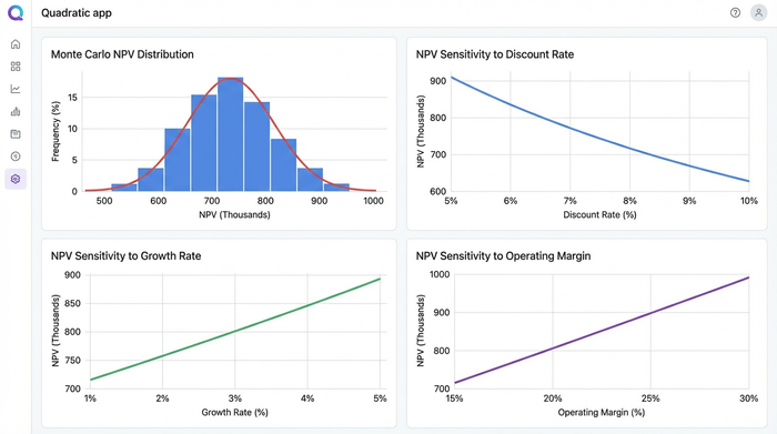
Perform sensitivity analysis. Always test how sensitive your NPV is to changes in the discount rate or terminal value, a process known as Sensitivity Analysis. Using Python loops, you can run thousands of scenarios in seconds to generate a distribution of possible outcomes, such as with Monte Carlo simulation, giving you a better grasp of the risk involved.

Ensure compliance. If your deal involves specific regulatory requirements, such as the acquisition of assets vs. business combination tax reporting, ensure your outputs map directly to the necessary forms. Your model should generate a summary table that aligns with the reporting needs of your finance team, reducing the friction between analysis and filing.

Conclusion

Asset acquisition is a high-stakes game where the margin for error is slim. Relying on fragile, manual spreadsheets to model complex deals limits your ability to analyze scenarios effectively and increases the risk of costly errors.

By moving beyond the limitations of traditional spreadsheets and embracing a modern modeling environment like Quadratic, you gain the power of Python, the flexibility of an infinite canvas, and the familiarity of a grid. You can build models that are not only powerful and dynamic but also fully transparent and auditable.

Whether you are evaluating a small portfolio purchase or a massive corporate transaction, the quality of your decision-making depends on the quality of your tools. Start building your asset acquisition model in Quadratic today for free, and experience the difference of a workflow designed for modern financial analysis.

Use Quadratic for Asset Acquisition Modeling

Use Quadratic to build robust and transparent financial models for asset acquisition:

• Build auditable models: Combine the familiar spreadsheet grid with Python's transparency and computational power to ensure your acquisition logic is clear and your path to NPV and IRR is verifiable.
• Automate complex deal structures: Elegantly switch between asset acquisition and business combination tax implications using Python variables, eliminating fragile IF statements and ensuring accurate depreciation schedules.
• Streamline input management: Query live data directly into your model using SQL or Python, centralizing inputs in a dynamic data frame that updates instantly without manual copy-pasting.
• Model operational scenarios with precision: Define revenue and cost functions using Python, making your operational forecasts transparent, scalable, and free from error-prone formula dragging.
• Perform precise investment appraisals: Calculate Net Present Value (NPV) and Internal Rate of Return (IRR) using self-documenting Python libraries, ensuring trustworthy financial metrics for confident decision-making.
• Visualize and compare scenarios instantly: Place multiple acquisition models side-by-side on the infinite canvas and use dynamic Python charts for real-time sensitivity analysis of base, optimistic, and pessimistic cases.
• Enhance model auditability: Document your logic directly within Python code and perform comprehensive sensitivity analysis with Python loops, ensuring compliance and reducing the risk of costly errors.

Start building your asset acquisition model today. Try Quadratic