
Equity valuation is the cornerstone of investment analysis. Whether you are a buy-side analyst, a portfolio manager, or a finance student, the ability to determine the intrinsic value of a company is critical. However, the traditional process of modeling is often plagued by manual data entry, brittle spreadsheets, and version control nightmares. Most analysts spend more time fixing broken links than they do analyzing the business.
Discounted cash flow models are widely considered the gold standard for estimating the value of an investment based on its expected future cash flows. The logic is sound, but the execution has historically been painful. A typical discounted cash flow model in Excel requires manually copying historical data from financial statements or PDF filings. This process is prone to error and difficult to audit.
The solution lies in moving from static inputs to dynamic modeling. By using Quadratic, you can build a model that pulls data programmatically and handles complex assumptions with transparency. This approach transforms the DCF from a static snapshot into a living tool that updates instantly as new data becomes available.
What is the discounted cash flow model?
Before diving into the mechanics of building a dynamic workflow, it is important to understand the core financial theory. A discounted cash flow valuation model relies on the time value of money, which is the principle that a dollar today is worth more than a dollar tomorrow due to its potential earning capacity.
To build this model, you generally need to calculate three specific components:
1. Free Cash Flow (FCF): This is the cash a company generates after accounting for cash outflows to support operations and maintain its capital assets.
2. Terminal Value: Since companies are assumed to operate indefinitely, you must estimate the value of the company beyond the projection period (usually 5 to 10 years).
3. Discount Rate (WACC): The Weighted Average Cost of Capital is the required rate of return used to bring those future cash flows back to their present value.
If you are asking what is the discounted cash flow model at its simplest level, it is a summation of these future cash flows, discounted back to today, to arrive at an Enterprise Value.
Step-by-step: Building a dynamic DCF model
In this walkthrough, we will follow the workflow of a modern financial professional. Instead of opening a blank sheet and typing numbers from a 10-K report, we will build a model that connects directly to data sources. This method ensures accuracy and saves hours of manual work.
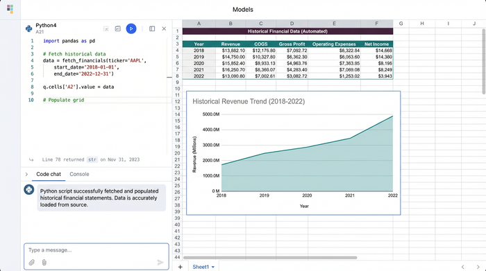
1. Automating historical data collection
The old way of modeling involved manually typing revenue, COGS, and operating expenses into a spreadsheet. This is where fat-finger errors happen. If the historical data is wrong, the entire valuation is flawed.
In Quadratic, you can automate this step. By using built-in SQL or Python integrations, you can fetch historical financial data directly into the grid. For example, you can write a simple query to pull the last five years of income statements and balance sheets for a specific ticker symbol. This data populates your cells automatically. The benefit is immediate: your model's starting point is always accurate, and updating the model for a new quarter is as simple as re-running the query.
2. Projecting revenue and margins
Once the historical data is in place, the next step is setting up assumptions for growth rates and operating margins. This is where the analyst's judgment comes into play. You will project future Free Cash Flows for a forecast period, typically 5 to 10 years.
In a dynamic environment, you can reference your historical data cells directly in your projection formulas. If you are building a simple discounted cash flow model, you might assume a constant growth rate. for more complex models, you can use Python to script distinct growth phases (high growth, transition, and stable growth).
A key tip here is to separate your "Inputs" from your "Calculations." In Quadratic, you can keep your assumptions in a clear, labeled section. Because the data flow is automated, you can instantly see how changing a revenue growth assumption from 5% to 8% impacts the bottom line without tracing through hidden formula chains.
3. Determining the discount rate (WACC)
The discount rate is often the most sensitive part of the model. Calculating the Weighted Average Cost of Capital involves several variables, including the Cost of Equity (calculated via CAPM), the Cost of Debt, and the company's capital structure.
In traditional spreadsheets, WACC calculations often result in long, nested formulas that are difficult to debug. Quadratic allows you to use Python variables for these inputs. You can define risk_free_rate, beta, and market_risk_premium as variables in a code cell. This makes the math easy to read and audit. Anyone reviewing your model can look at the code and understand exactly how the discount rate was derived.
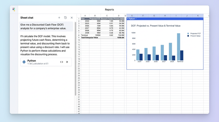
4. Calculating terminal value and present value
There are two primary methods to calculate Terminal Value: the Gordon Growth Method and the Exit Multiple Method). A robust discounted cash flow model example will often calculate both to provide a valuation range.
Using the Gordon Growth Method, you assume the company grows at a stable rate forever after the projection period. Using the Exit Multiple Method, you apply an industry-standard multiple (like EV/EBITDA) to the final year's metric.
Once you have the projected FCFs and the Terminal Value, you discount them back to the present day using the WACC calculated in the previous step. The sum of these present values gives you the Enterprise Value.
5. Deriving the implied share price
The final step bridges the gap between Enterprise Value and the specific value of the equity. To do this, you subtract Net Debt (Total Debt minus Cash) from the Enterprise Value to arrive at the Equity Value.
Finally, divide the Equity Value by the diluted share count. This yields the intrinsic share price. This output is the decision-making signal. If your model's implied share price is significantly higher than the current market price, it suggests the stock may be undervalued. Because you built this in Quadratic, you can trust that the signal is based on live data and transparent logic, not a hard-coded number from a broken link.
Best practices for building a discounted cash flow DCF model
Building a model is not just about getting a number; it is about building a tool that can withstand scrutiny. Adhering to best practices for building a discounted cash flow DCF model ensures your work is defensible and reusable.
Moving beyond "discounted cash flow model Excel" limitations
The most common criticism of a standard discounted cash flow model Excel file is its lack of auditability. Formulas are hidden inside cells, and logic is often obscured. In Quadratic, you can use Python for complex logic, making the model readable for colleagues. A block of code explaining the tax rate calculation is far superior to a cell containing =IF(B2>0, B2*0.21, 0).
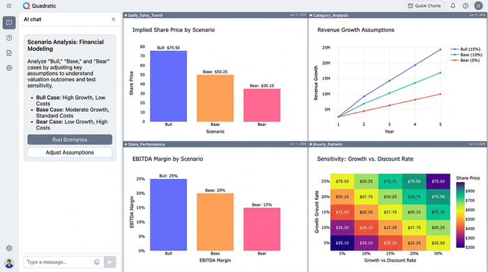
Scenario analysis is another critical best practice. A robust model should never rely on a single set of assumptions. You should be able to stress-test your valuation. By using variables for your "Bull," "Base," and "Bear" cases, you can toggle between scenarios instantly to see how sensitive your valuation is to changes in revenue growth or WACC.
Finally, focus on templating. In a traditional workflow, using an old model for a new company involves a dangerous amount of deleting and replacing data. In Quadratic, because the data fetch is automated, you can create a reusable discounted cash flow model template. By simply changing the ticker symbol in your input cell, the Python or SQL query will fetch the new company's data, and the entire model will update automatically. This allows you to value a dozen companies in the time it used to take to value one.
Conclusion
Building a DCF is about understanding the business and making informed predictions, not fighting with spreadsheet cells. The logic of valuation remains constant, but the tools we use to execute it have evolved.
By moving from static manual entry to dynamic modeling in Quadratic, analysts can eliminate the drudgery of data maintenance. You gain the ability to audit your logic clearly, update data instantly, and reuse your work across different companies. Whether you are building your first model or refining a complex institutional template, the shift to a dynamic workflow allows you to focus on what matters most: the strategy behind the valuation.
If you are ready to modernize your analysis, you can start building your own valuation models in Quadratic today or download a starter discounted cash flow model template to experiment with the power of Python and SQL in your grid.
Use Quadratic to build discounted cash flow models
- Automate historical data collection: Connect directly to financial data sources with Python or SQL to pull historical financials, eliminating manual entry and ensuring accuracy.
- Build dynamic, self-updating models: Transform static DCF models into living tools that instantly refresh with new data and reflect assumption changes.
- Enhance auditability and transparency: Clearly define complex calculations like WACC and projections using readable Python code and separate input sections.
- Streamline scenario analysis: Easily stress-test valuations by toggling between different growth rates, margins, and discount rate assumptions.
- Create reusable valuation templates: Build models that update automatically for new companies by simply changing a ticker, saving significant time and effort.
Ready to modernize your financial analysis? Try Quadratic.