NBA DFS projections: crafting accurate player values

In the competitive world of NBA Daily Fantasy Sports (DFS), relying on the same free NBA DFS projections as the rest of the field is often a recipe for breaking even or splitting pots. Serious players eventually hit a ceiling with this approach. They either find themselves paying for expensive "black box" subscription tools they cannot customize, or they get stuck in "Excel Hell"—manually copy-pasting game logs, wrestling with broken formulas, and running out of time before lock.

To find a true edge, you need to move from consuming data to creating it, a foundational aspect of modern sports analytics. This article walks through a real analyst’s workflow using Quadratic, a tool that combines the visual interface of a spreadsheet with the automation of Python. By the end, you will understand how to build a transparent "White Box" system to generate the best NBA DFS projections that update automatically, giving you the control to find value where others miss it.

Why build your own projection model?

The primary advantage of building your own model is the ability to pivot away from consensus. When you rely solely on public tools, you are often pushed toward "chalk"—highly owned players that everyone else is drafting. If those players fail, your lineup sinks with the majority. By building your own NBA projections DFS system, you can tweak variables to find contrarian value.

Furthermore, transparency is critical for long-term success. If a subscription tool projects a player for 40 fantasy points, you rarely know why. Is it based on a pace uptick? A usage increase due to a teammate's injury? Or is it a data error? When you build the logic yourself, you know exactly why a player is popping in your model.

This is where the hybrid approach of Quadratic becomes essential. Standard spreadsheets often struggle with the complexity of DFS projections NBA workflows. They require distinct sheets for team stats, player data, and analysis, all linked dynamically. Traditional VLOOKUP or INDEX/MATCH formulas can become fragile and slow when processing thousands of rows of game logs daily. A hybrid tool allows you to keep the spreadsheet interface for viewing data while using Python for the heavy lifting, ensuring your model is both powerful and transparent.

Step 1: Data ingestion and organization

The foundation of any robust model is clean, automated data. In a manual workflow, you might spend the first hour of your day downloading CSVs to get NBA DFS projections today. In this modern workflow, data ingestion is automated.

The workspace is typically organized into three distinct areas:

1. Raw Data: This sheet houses historical game logs and live betting market lines.

2. Team Stats: This area aggregates team-level metrics like pace of play and defensive rating.

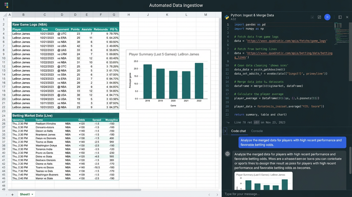
3. Analysis: This is the staging ground where the calculations and projections happen.

Using Quadratic, you can use Python directly within the cells to fetch data via sports data APIs (such as BallDontLie or sports data aggregators) or scrape public datasets. Instead of pasting data every morning, a simple script refresh pulls the latest game logs and betting lines instantly.

This automation solves a major pain point: data blending. Merging "Historical Stats" with "Live Betting Markets" is notoriously difficult in standard spreadsheets because player names often differ between sources (e.g., "CJ McCollum" vs. "C.J. McCollum"). Python libraries like Pandas—which run natively in Quadratic—can handle fuzzy matching and merging cleanly, ensuring your base data is accurate without manual intervention.

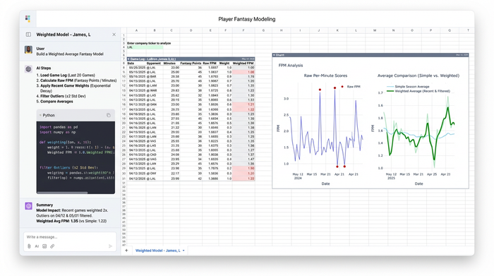
Step 2: Calculating weighted per-minute rates

Once the data is ingested, the core data modeling begins. A common mistake is relying on per-game averages. In the NBA, minutes played are the most volatile variable, while per-minute production is generally more stable. Therefore, the most accurate NBA DFS player projections rely on calculating a player's Fantasy Points Per Minute (PPM) and then applying that rate to their projected minutes.

However, not all historical data is equal. A game from October is less relevant than a game from last week, especially if the team rotation has changed. In this workflow, you can apply "Weighted Historical Rates." Using a Python script within the sheet, you can apply a decay function that weights the last 10 games significantly heavier than the previous 50. This captures a player's current form or recent role change—such as a bench player stepping into the starting lineup—much faster than a simple season-long average.

Additionally, Python allows for sophisticated outlier filtering. You can program the model to automatically exclude games where a player played fewer than five minutes (due to injury or ejection) or "garbage time" minutes. This ensures your baseline PPM calculation isn't skewed by irrelevant data points, resulting in a cleaner, more reliable projection.

Step 3: Contextual adjustments (defense & pace)

Raw statistical projections are only the starting point. To create truly sharp DFS NBA projections, you must adjust for the specific context of that night's slate. Two massive factors drive these adjustments: defensive strength and game pace.

First, the model must account for the opponent. If a player is facing a top-tier defense that allows the fewest fantasy points to their position, your model should scale their projection down. Conversely, a matchup against a weak defense warrants a boost.

Second, pace factors are critical. The NBA is a game of possessions. Using the "Market-Implied Game Pace" derived from betting totals, you can adjust expectations. If the betting line suggests a high-scoring, fast-paced shootout, the model scales up projections for all players in that game because there will simply be more opportunities to score fantasy points.

Finally, many pros use a "Composite" approach. This involves blending your calculated internal projection with third-party expert baselines. By averaging your custom numbers with an external source, you smooth out volatility and reduce the risk of a massive outlier ruining your lineup.

Step 4: Finding value (EV+) and ownership leverage

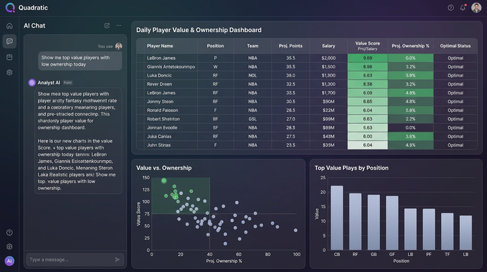
With a refined projection in hand, the focus shifts to execution. The goal is to identify where your model disagrees with the market.

One of the strongest indicators of value is comparing your internal projection against live betting lines (player props). If your model projects a player for 25 points, but the sportsbook has the line set at 19.5, you have identified a significant edge. This discrepancy suggests that the player is undervalued relative to the market's expectation.

In DFS, this translates to "Value"—typically calculated as projected points per dollar of salary. But to win tournaments, you also need to consider NBA DFS ownership projections. The "Tournament Winning" play often occurs when your model loves a player that the public hates. If your data indicates a player is a top value, but DFS ownership projections NBA show them at less than 5% ownership, you gain massive leverage on the field by rostering them. This combination of high projection and low ownership is the holy grail of DFS strategy.

Why Quadratic is the best tool for DFS modeling

The workflow described above is difficult to maintain in legacy spreadsheets and too abstract to visualize in a pure code editor. Quadratic bridges this gap, making it the ideal environment for creating the best NBA DFS projections.

The ability to run Python directly in the grid allows for complex weighting algorithms and fuzzy matching, such as those used in the analytic hierarchy process, that standard formulas cannot handle. Because the data connections are live, your model updates as betting lines move throughout the day, ensuring you are never making decisions based on stale information. Most importantly, you retain the visual clarity of a spreadsheet, allowing you to create a dashboard in Python for your data. You can see the rows, filter the columns, and verify the logic instantly, giving you full confidence in the numbers you are betting on.

Conclusion

Building free NBA DFS projections systems yourself, much like in fp&a modeling, yields significantly better long-term results than relying on static lists or expensive subscriptions. By taking control of the data, you understand the "why" behind every pick.

By combining historical data, market signals, and weighted algorithms in a single dynamic workspace, you stop guessing and start investing, much like in financial valuation. You move from a player who hopes for luck to an analyst who engineers an edge. Start building your automated NBA model in Quadratic today to turn raw stats into actionable value.

Use Quadratic to build custom NBA DFS projections

• Automate data ingestion and blending: Pull live game logs and betting lines with Python scripts directly in the grid, eliminating manual copy-pasting and fuzzy matching issues.
• Build sophisticated projection models: Apply weighted historical rates, decay functions, and outlier filtering with native Python, ensuring accurate per-minute fantasy point calculations.
• Make real-time contextual adjustments: Dynamically factor in opponent defensive strength, market-implied game pace, and blend with third-party baselines using Python for sharper projections.
• Identify value and leverage instantly: Compare your projections against live betting lines and assess ownership data in a visual spreadsheet environment to find profitable opportunities.
• Maintain transparency and control: Combine the visual clarity of a spreadsheet with the power of Python, allowing you to see, verify, and customize every piece of your projection logic.

Start building your automated NBA DFS model today. Try Quadratic.