Mastering product profitability analysis for complex projects

For modern financial analysts, product profitability analysis is rarely as simple as subtracting costs from revenue. While the basic formulas are straightforward, the reality of business is messy. Analysts are often tasked with building multi-year projections that must account for changing variables, massive datasets, and shifting operational timelines.

Standard spreadsheets are excellent for simple profit and loss statements, but they often become fragile when modeling complex scenarios. A common example is a manufacturing plant relocation or a multi-product line expansion where cost structures change mid-stream. When you try to force these dynamic timelines into static spreadsheet cells, you end up with "spaghetti code"—a fragile web of dependencies that breaks the moment a variable changes.

To solve this, financial professionals are moving from static modeling to dynamic data modeling using tools like Quadratic. By combining the familiarity of a coding spreadsheet with the power of Python and SQL, you can build robust viability models that handle granular data inputs and complex timeline logic without breaking. This approach allows you to focus on the strategy behind the numbers rather than debugging broken formulas.

What is product profitability analysis? (The baseline)

Before diving into complex workflows, it is helpful to establish a baseline product profitability analysis definition. It is the process of evaluating the financial viability of a specific product or product line by attributing direct costs, indirect costs, and capital expenditures to revenue streams. The goal is to understand not just if the company is making money, but specifically which products are driving value and which are draining resources.

To get a clear picture, analysts rely on several essential product profitability analysis metrics:

• Gross Margin & Contribution Margin: These measure the revenue remaining after direct costs and variable costs are deducted.
• Break-even Point: This is crucial for cost volume profit analysis for multiple products, helping teams understand how many units must be sold to cover costs.
• Return on Investment (ROI) and Payback Period: These metrics track how long it takes for the profit from a product to repay the initial capital investment.

While these concepts are fundamental, there is often a gap between theory and practice. A static product profitability analysis example might show a clean, linear projection. However, in the real world, a five-year project might involve fluctuating raw material costs, a mid-project facility move, and changing overhead allocations. This is where standard templates fail and dynamic modeling becomes necessary.

The challenge: modeling phased operational changes

Consider a specific, complex use case: a financial analyst modeling the viability of a multi-year manufacturing project. The project involves producing and selling a specific widget, but there is a catch. The manufacturing will start at "Facility A" (an older, higher-cost plant) and, after 18 months, relocate to "Facility B" (a new, capital-intensive but lower-operating-cost plant).

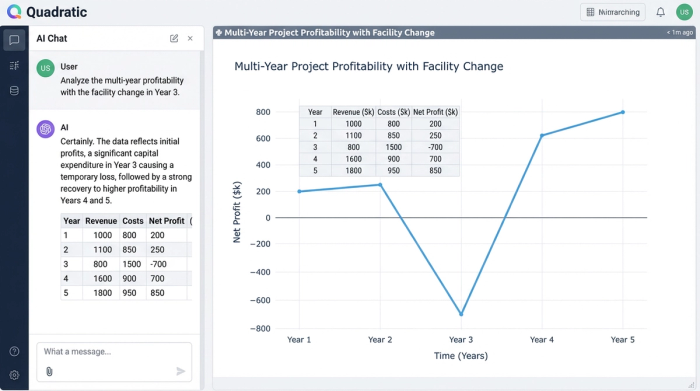
This introduces "phased complexity." In a standard product profitability analysis excel template, handling this transition is a nightmare. You might find yourself writing massive, nested IF/THEN statements to tell the model to switch cost structures on a specific date. You have to account for:

• The switch from "Old Facility" overheads to "New Facility" overheads.
• Amortizing the Capital Expenditure (CapEx) of the new facility only after it becomes operational.
• Fluctuating logistics costs during the transition period.

When you try to perform product line profitability analysis under these conditions using only standard cell formulas, the model becomes rigid. If the relocation date slips by three months, you might have to manually update columns of formulas, increasing the risk of human error.

Step 1: Automating granular data ingestion

The first step to mastering this complexity is improving how data enters your model. In traditional workflows, analysts often manually paste raw material costs, administrative drivers, and sales prices into an "Assumptions" tab. This data quickly becomes stale, and tracing the source of a specific cost assumption can be difficult.

In Quadratic, you can automate this process. Instead of manual entry, you can use SQL to pull live cost data directly from your database or use Python to map consistent data structures into the grid. For example, you can ingest a raw dataset containing historical raw material prices and projected labor rates.

By automating this ingestion, you ensure that your customer and product profitability analysis is based on validated, up-to-date inputs. You are no longer aggregating data prematurely; you are bringing in the granular details—such as specific administrative expense drivers or distinct CapEx line items—and letting the model handle the aggregation. This creates a "single source of truth" within your spreadsheet that updates automatically when the underlying data changes.

Step 2: Handling complexity with Python logic

Once the data is in the grid, the next challenge is managing the logic for the facility relocation. This is where the hybrid nature of Quadratic transforms the workflow. Instead of hiding the logic in a complex chain of Excel formulas, you can use Python directly within the cells to handle the phased changes.

For the manufacturing use case, the analyst can write a clean Python script to calculate costs based on the timeline. The logic might look something like this:

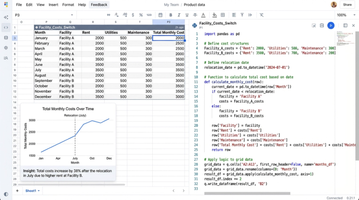
• If the current date is before the Relocation Date, use Facility A's cost structure (higher opex, zero new CapEx depreciation).
• If the current date is on or after the Relocation Date, use Facility B's cost structure (lower opex, plus amortized CapEx).

Because this logic is written in code, it is readable and auditable. You can clearly see the "switch" happening in the script. If the project lead decides to delay the move by six months, you simply update the "Relocation Date" variable, and the Python script automatically recalculates the entire timeline. This makes the model resilient and allows for sophisticated customer product profitability analysis that accurately reflects operational reality.

Step 3: Analyzing viability and payback

With the data automated and the logic streamlined, the model can now aggregate the granular inputs into a final financial view. This is where you assess the true viability of the project. You can see exactly how the initial high costs of Facility A impact cash flow and how quickly the efficiency gains of Facility B pay back the investment.

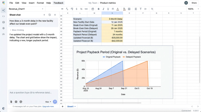
This dynamic setup is perfect for scenario planning and performing sensitivity analysis. You can instantly answer questions like, "What happens to our margins if raw material costs rise by 5% during the transition?" or "How does a delay in the new facility affect our break-even point?"

This capability is essential when performing multiple product cost volume profit analysis. You can model different product lines running through these facilities simultaneously to see which products sustain the business during the high-cost transition period and which ones maximize profit once the new facility is online.

Best practices for robust financial modeling

To truly master product profitability analysis, it is important to adopt a "Data Ops" mindset, even within a spreadsheet environment.

• Consistent Data Mapping: Ensure all inputs, from CapEx details to administrative expenses, follow a strict schema. This prevents the model from breaking when new data is added.
• Auditability: Keep your logic visible. Using Python or SQL for complex transformations is safer than hiding logic in cell dependencies that are hard to trace, contributing to more auditable financial models.
• Dynamic vs. Static: Move away from static product profitability analysis examples that only show a snapshot in time. Build models that react to live business changes.

By following these best practices, you ensure that your analysis is not just a one-off calculation, but a durable tool that can guide decision-making throughout the project's lifecycle.

Conclusion

Complex projects like manufacturing relocations or multi-year expansions require more than just a standard spreadsheet; they require a tool that understands logic and data flow. By using Quadratic, financial analysts can bridge the gap between static templates and full-scale data applications.

Mastering product profitability analysis is about more than knowing the formulas—it is about building models that can withstand the pressure of real-world variables. With the ability to automate data ingestion and handle phased logic with Python, you can deliver insights that are accurate, auditable, and actionable.

Try Quadratic to model your next complex project and experience the difference of a spreadsheet built for modern data analysis.

Use Quadratic to do product profitability analysis

• Model complex, multi-year product profitability scenarios with dynamic timelines, such as phased facility changes, without fragile spreadsheet formulas.
• Automate the ingestion of granular cost data (like raw materials, labor rates, and CapEx) directly from databases using SQL or Python for consistently up-to-date inputs.
• Implement sophisticated operational logic, such as switching cost structures based on specific dates, directly in cells with readable Python scripts.
• Easily perform scenario planning and sensitivity analysis by updating key variables, instantly recalculating the entire model for different outcomes.
• Build auditable and resilient profitability models that adapt to real-world changes, eliminating manual formula adjustments and reducing the risk of error.

Ready to build more robust profitability models? Try Quadratic.