Every pile foundation is, at its core, a load transfer problem. Structural loads from columns and walls must travel down through soft, compressible surface soils until they reach a competent bearing stratum capable of carrying them safely. Getting that capacity calculation right is non-negotiable, and the consequences of error show up quickly in the field — excessive settlement, refusal during driving, or worse.
Yet for all its importance, pile driving analysis still lives in a fragmented toolset. Geotechnical theory sits in academic PDFs and reference manuals. Specialized wave equation programs run in their own silos. And the day-to-day capacity calculations happen in a messy excel sheet that engineers inherit, modify, and rarely fully trust.
This article walks through a different approach: a civil engineer's end-to-end pile foundation workflow built inside Quadratic, where static soil analysis, structural compliance checks, and design documentation all live in a single canvas.
What is pile driving analysis?
Before getting into the workflow, it helps to ground the terminology, since the phrase covers more than one engineering activity.
Defining pile driving analysis
Pile driving analysis is the engineering process of evaluating pile capacity, drivability, and load transfer mechanisms during foundation design. In practice, it splits into two related but distinct branches.
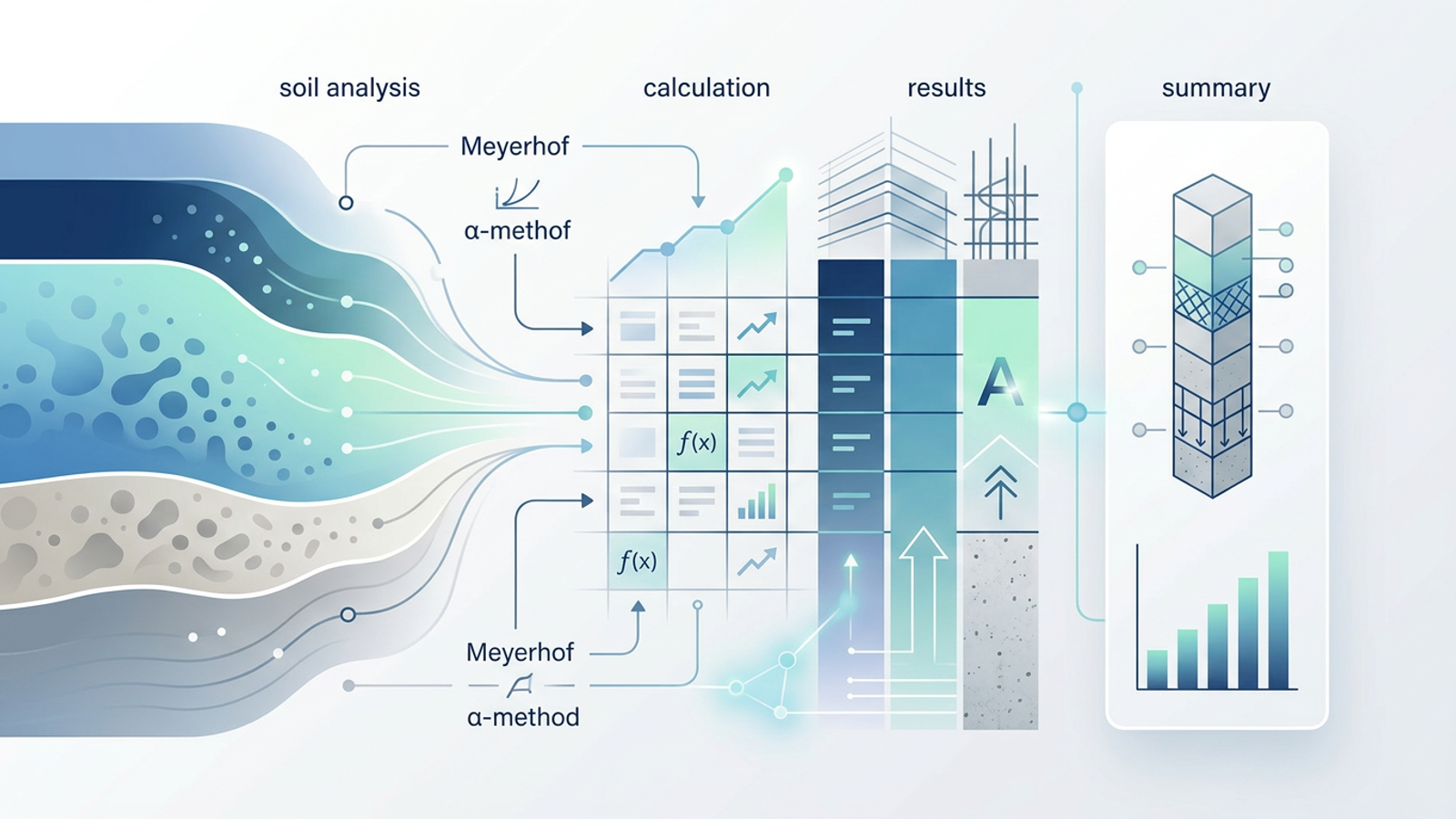
Static analysis estimates ultimate and allowable pile capacity from soil parameters — unit weight, cohesion, friction angle, SPT N-values — using established methods like Meyerhof for sand and the α-method for clay. This is the design-phase calculation that determines how many piles you need and how long they have to be.
Dynamic analysis, often referred to as pile driving analysis by the wave equation, models the pile, hammer, and soil as a one-dimensional stress wave problem. Programs based on Smith's wave equation simulate hammer blows to predict drivability and bearing capacity. In the field, the same theory underpins PDA testing, where instrumented piles are monitored during installation.
The pile driving analysis test and test procedure
A pile driving analysis test, commonly called a PDA test, is a field validation method that measures force and velocity at the pile head using strain gauges and accelerometers attached near the top of the pile.
The standard pile driving analysis test procedure involves instrumenting the pile, capturing data from a series of hammer blows, and applying the Case Method in real time to estimate capacity. Recorded blows are later refined using CAPWAP signal matching, which iteratively adjusts soil resistance distribution until the simulated response matches the measured one.
A pile driving analysis system — the integrated hardware and software used during the test — ties those field measurements back to the predicted static capacity established during design. The static numbers calculated at the desk become the targets the field test is asked to validate.
The core equations every engineer calculates
The design-phase math is well established. Most static capacity work reduces to a handful of equations applied across soil layers.
Ultimate pile capacity
The universal expression for ultimate pile capacity is:
Qu = Qp + Qs
Where Qp is end bearing at the pile tip and Qs is the cumulative skin friction along the pile shaft. Dividing ultimate capacity by a factor of safety (typically 2.5 to 3.0) yields the allowable capacity used in design.
Meyerhof's method for sandy soils
In cohesionless soils, Meyerhof's method estimates end bearing from SPT N-values:
Qp = 40 · N · L/D · Ap ≤ 400 · N · Ap
Skin friction in sand is similarly tied to N-values, typically expressed as fs = 2 · N (in kPa) for driven piles, summed over the embedded length.
The α-method for clay
In cohesive soils, skin friction is calculated using an adhesion factor applied to undrained shear strength using the total stress approach (commonly known as the α-method):
fs = α · cu
End bearing in clay follows:
Qp = 9 · cu · Ap
The adhesion factor α depends on cu and pile type, and is typically read from published correlations.
Where traditional spreadsheets fall short
None of this math is exotic. When engineers try to explain excel spreadsheet models inherited from past projects, they find that formulas get buried, scenario testing requires duplicating sheets, and drawings have to be generated in separate tools. The pain comes from executing it across a layered soil profile, switching methods by layer, integrating structural specifications, running scenario tests on pile diameter and length, and then producing client-ready documentation.
A real pile foundation workflow in Quadratic
Here is how a civil engineer designing pile foundations for a construction project can run the entire workflow in one Quadratic file.
Setting up the soil profile
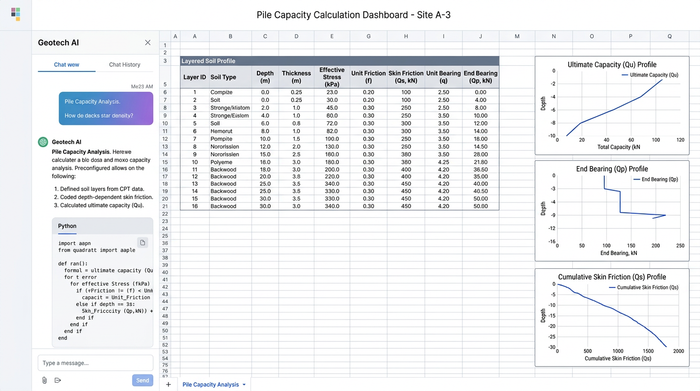
The engineer starts by entering layered soil data directly into the grid: depth intervals, soil type, unit weight, cohesion, friction angle, and SPT N-values for each stratum. Borehole logs from multiple locations can be pasted in or imported, with each layer becoming a row that downstream formulas reference.
Because Quadratic handles large datasets without the lag that plagues older spreadsheet tools, engineers can keep the full borehole log live in the sheet rather than summarizing it into a stripped-down input table.
Calculating pile capacity with Meyerhof and the α-method
With the soil profile in place, capacity formulas are implemented as cell-based calculations layer by layer. For sand layers, Meyerhof's expressions for unit skin friction and end bearing reference the SPT N-values directly. For clay layers, the α-method pulls undrained shear strength and applies the appropriate adhesion factor.
A simple conditional column lets the engineer flag each layer as cohesive or cohesionless, so the correct method is applied automatically. Skin friction contributions are summed cumulatively with depth, giving Qs at any candidate pile length. End bearing is computed at the pile tip using the properties of the bearing layer.
The result is a single table where pile length is an input and Qu, Qp, and Qs update instantly.
Applying the factor of safety and required pile count
Allowable capacity is derived by dividing Qu by the chosen factor of safety. Total structural load from the superstructure is then divided by the allowable capacity per pile to determine the required pile count.
Because every value is connected through cell references, the engineer can iterate quickly: change the pile diameter from 400 mm to 500 mm, sweep length from 12 m to 25 m, or adjust the FOS, and the required pile count updates across the sheet. This is where Quadratic's responsiveness pays off — scenario testing that would feel sluggish in a legacy template runs immediately.
Integrating structural specifications (concrete and rebar)
This is where the fragmentation gap actually closes. In the same canvas, the engineer adds the structural design parameters: concrete compressive strength (f'c), rebar grade and area, cover requirements, and the resulting structural axial capacity of the pile section.
A side-by-side comparison checks structural capacity against geotechnical capacity to identify which governs. Code references — ACI 318 for concrete design, IBC for load combinations, or the relevant regional standard — sit alongside the calculations so reviewers can trace each value back to its source. If the structural section governs, the engineer knows to increase reinforcement or section size; if geotechnical capacity governs, longer or larger piles are the lever.
Generating engineering drawings and design documentation with Python
The final piece is documentation. Quadratic's native Python integration lets the engineer drop matplotlib code directly into a cell to render visuals from the same data that drives the calculations.
A typical setup includes a pile cross-section showing concrete dimensions and rebar layout, a soil profile diagram annotated with layer properties and the pile embedded through them, and a load distribution chart plotting cumulative skin friction and end bearing along depth. Because the plots read from the same cells as the capacity calculations, any change to pile geometry or soil parameters propagates through to the figures automatically.
Alongside the diagrams, a summary table consolidates the deliverables: pile diameter and length, allowable capacity, factor of safety, governing failure mode, structural reinforcement, and code references. No exporting to a separate CAD tool for preliminary drawings, no copy-pasting numbers into Word, no broken links between calculation files and report figures.
Why Quadratic outperforms legacy spreadsheet tools for foundation design
A few characteristics make this workflow practical in Quadratic where it would be painful elsewhere.
Performance is the baseline. Multi-layer soil calculations with dozens of dependent formulas run without the recalculation lag that older tools impose on large engineering workbooks.
Programmability is the multiplier. Because Quadratic operates as a native python spreadsheet, engineers can automate parametric studies — sweep pile lengths from 10 m to 30 m, generate capacity curves, run sensitivity analyses on friction angle or cohesion — without leaving the sheet. SQL connections let teams pull soil data directly from project databases, streamlining data analysis using excel and sql.
The spatial canvas keeps everything visible. Calculations, code references, soil tables, structural checks, and rendered drawings coexist on the same surface instead of being scattered across files, tabs, and external tools. Reviewers can follow the design from input to figure in one place.
Real-time multiplayer collaboration also matters on engineering teams, where a geotechnical engineer, structural engineer, and project manager often need to look at the same numbers at the same time. A shared Quadratic file replaces the email chain of versioned attachments.
From static analysis to field validation
The static analysis produced in Quadratic does not end at the desk. The allowable capacity values calculated from Meyerhof and the α-method become the design targets that a pile driving analysis system validates in the field.
When PDA equipment is set up on site and the pile driving analysis test procedure begins, field engineers compare measured capacity against the predicted values from the design workbook. A well-documented Quadratic file — soil profile, governing assumptions, predicted Qu, structural capacity, code references — becomes the source of truth that anchors the validation conversation. If field results diverge significantly from predictions, the design model is right there to interrogate and update.
That closes the loop between design and construction, which is exactly where fragmented toolchains tend to break down.
Conclusion
Pile driving analysis touches geotechnical theory, structural design, and engineering documentation. Traditionally, engineers have had to stitch those three domains together across academic references, standalone wave equation programs, brittle Excel templates, and external drafting tools.
The workflow described here — soil profile, Meyerhof and α-method capacity calculations, factor of safety and pile count, concrete and rebar checks against building codes, and Python-generated diagrams and summary tables — all happens in one Quadratic file. The math is the same math engineers have always done. What changes is the friction around it.
If you design pile foundations, open Quadratic and try replicating a section of your current workbook in the canvas. Bring in a borehole log, set up the capacity formulas, and add a matplotlib cross-section next to the numbers. The seams between calculation, compliance, and documentation start to disappear once everything shares the same workspace.
Use Quadratic to do pile driving analysis
- Keep entire borehole logs live in your sheet without the performance lag or formula delays of legacy spreadsheets.
- Apply Meyerhof and α-method capacity calculations automatically across cohesive and cohesionless soil layers using conditional logic.
- Run immediate scenario testing on pile diameter, length, and factors of safety to see required pile counts update instantly.
- Compare structural axial capacity against geotechnical capacity on a single canvas, keeping your code references and calculations side by side.
- Generate live soil profiles, pile cross-sections, and capacity curves using native Python and matplotlib right next to your grid data.
- Share a single, real-time workspace with structural engineers, project managers, and field testing teams to bridge the gap between design and site validation.
Ready to streamline your foundation design workflow? Create a free account and Try Quadratic