James Amoo, Community Partner
Jun 1, 2026

You have built a Monte Carlo simulation Excel workflow before. You wired up RAND across your assumption cells, stretched a Data Table down ten thousand rows, watched the workbook freeze for thirty seconds, and then realized that pressing F9 to refresh produced a slightly different distribution every time. The model almost works. It just feels brittle in ways that are hard to articulate to whoever asked for it.
Here is the thesis of this article: the pain of running a Monte Carlo simulation in Excel is a tool gap, not a skill gap. The friction analysts feel when they push Excel into iterative simulation is not a reflection of how well they understand probability, sampling, or finance. It is a reflection of the fact that Excel was designed for deterministic and single-pass calculation, and Monte Carlo asks for something fundamentally different.
In the sections below, we will examine the four specific mechanisms in which Excel Monte Carlo simulation breaks down. This includes volatile randomness, the misuse of Data Tables as iteration loops, the absence of seeding, and disconnected output charting. Then we will describe what a friction-free workflow actually looks like when those constraints are removed.
What Monte Carlo simulation require from a tool
What Monte Carlo simulation requires from a tool is fairly specific. It needs the ability to run many iterations, often tens or hundreds of thousands of trials, without performance collapsing. It requires controllable randomness, where distributions like normal and correlated inputs can be specified explicitly rather than approximated through cell tricks. It also depends on reproducibility, meaning the same seed and inputs must always produce the same output, so results can be audited or shared. Finally, it needs proper statistical outputs for predictive analytics.
Now contrast that with what spreadsheets were built for. Monte Carlo simulation, which relies on repeated random sampling to estimate outcomes across uncertain systems, sits in tension with Excel’s core model of single-pass recalculation across a dependency graph. Each cell is designed to compute a stable result from defined inputs, not to execute thousands of stochastic iterations as a primary workload. While Excel can approximate simulation using functions like RAND and replicated rows, the model is essentially being forced to behave like a simulation engine it was never designed to be. That works for small-scale experiments, but it breaks down in performance and interpretability as models grow.
This is where Quadratic becomes relevant, because it is designed to treat simulation as a first-class workload rather than a spreadsheet hack. By combining Python, SQL, and spreadsheet grids in one environment, Quadratic allows Monte Carlo models to run as real code while still rendering results in a familiar tabular interface. That means you can define distributions, run vectorized simulations, and compute statistical summaries in a way that is both performant and reproducible, while still keeping outputs inspectable in a grid. It also offers a Monte Carlo simulation Excel template free for use.
Where Excel breaks down for Monte Carlo simulation
Analysts often explore how to do Monte Carlo simulation in Excel, but it breaks down when things get too complex. Let’s explore some of the limitations of Excel.
RAND and RANDBETWEEN: volatility without control
RAND and RANDBETWEEN are volatile functions, a recalculation behavior that sits fundamentally at odds with how Monte Carlo methods are designed to operate. They recalculate on every edit, every workbook open, every F9 press, and every save. For a normal spreadsheet, that is fine. For a Monte Carlo simulation with Excel, it is corrosive.
The moment you nudge an unrelated cell, your entire simulation reshuffles. The histogram you screenshotted yesterday no longer matches the workbook you opened today. There is no native way to fix the random stream so it stays put while you finish documentation or walk a colleague through the model.
The downstream consequence is that you cannot reliably re-run the same scenario or audit a specific run after the fact. Every save is a new world.
Data tables: a sensitivity tool pressed into iteration duty
Most tutorials on how to run Monte Carlo simulation in Excel converge on the same workaround: use a one- or two-variable Data Table to "loop" thousands of trials, with each row index acting as a fake trial counter. The Data Table forces Excel to recalculate the model once per row, and you collect the output column as your sample.
It works, but the architecture is wrong. Data Tables were built for sensitivity analysis, not for iterative stochastic simulation. Repurposing them as iteration engines means the row index is not really a trial, and the recalculation cost scales linearly with iteration count.
The performance pain is real. Large Data Tables slow recalculation across the entire workbook and force you to keep iteration counts artificially low. Iteration count stops being a modeling decision based on how much precision you need and becomes a UX decision based on how much your laptop can tolerate.
No seeding, no reproducibility, no audit trail
Excel has no built-in mechanism to fix the random seed across runs. There are workarounds involving manual conversion of RAND outputs to static values via paste-special, but that defeats the purpose of a live simulation, and it does not let you re-run the same stochastic stream against a modified assumption.
For finance teams focused on the best financial reporting, this is not a minor inconvenience. Results that cannot be reproduced cannot be reviewed. A simulation that produces a slightly different 95th percentile every time you open the file is hard to defend, regardless of how sound the underlying logic is.
Manual charting and output summarization
The output side of an Excel Monte Carlo workflow is just as fragmented as the input side. Histograms require a separate FREQUENCY formula and a chart bound to fixed bin ranges. Percentile tables are their own block of PERCENTILE calls. Convergence plots, which show how the running mean stabilizes as iterations accumulate, are rarely built at all because they require even more manual scaffolding.
Every time you change the model, the chart ranges and bin boundaries have to be revisited. The output layer is structurally disconnected from the simulation layer, which means every model change increases the surface area for charting errors.
Distribution flexibility and sampling quality
RAND produces uniform draws on [0, 1). Anything else is a formula composition. Normal draws come from NORM.INV(RAND(), mu, sigma). Lognormal, triangular, beta, and empirical distributions each require their own assembly. Correlated draws across multiple inputs require Cholesky decomposition implemented in cells. Latin Hypercube and other variance reduction techniques are effectively off the table without significant custom work.
A Monte Carlo simulation Excel add in can patch some of this by providing distribution libraries, correlation matrices, and better output reporting. You take on vendor lock-in and a dependency that not every reviewer will have installed. The add-in still operates inside Excel's volatile recalculation model, so it inherits the reproducibility and performance constraints described above.
How Quadratic fits: spreadsheet structure, Python-powered simulation
Quadratic is a browser-based spreadsheet that runs native Python and SQL directly in the same grid as your formulas and cells. Your assumptions live where they always have, in labeled cells you can edit and reference. The simulation itself is written as Python code with full access to the rest of the sheet. Let’s explore the capabilities of Quadratic in detail.
Blend financial modeling, SQL, and simulation in one workflow
Many real-world forecasting workflows do not begin with manually entered assumptions. They begin with operational data pulled from databases using an Excel connect to SQL Server workflow, APIs, or recurring exports that feed directly into simulation models.
Quadratic supports live data connections alongside Python, formulas, and SQL in the same spreadsheet environment. That allows Monte Carlo models to operate against current operational data instead of isolated spreadsheet snapshots.
A SaaS finance team, for example, could query customer retention data from Snowflake using SQL data analytics, calculate cohort analysis with Python, simulate revenue outcomes under multiple pricing assumptions, and present forecast distributions in dashboards directly beside the source data.
Run reproducible simulations instead of volatile spreadsheet randomness
One of the biggest weaknesses in traditional Monte Carlo simulation Excel workflows is reproducibility. Excel's RAND function recalculates constantly, making it difficult to guarantee that the same assumptions generate the same output distribution across runs.
Quadratic resolves that issue through its coding spreadsheet support and explicit control over random seeds using numpy.random. Analysts can define a seed directly in the simulation logic, ensuring that a given set of assumptions produces the same distribution every time the model runs.
That capability matters operationally for finance, risk, and forecasting workflows where auditability is critical. A treasury team modeling cash flow exposure can preserve exact simulation conditions for review and future reruns instead of relying on volatile spreadsheet recalculation behavior.
Scale iteration counts without spreadsheet performance collapse
Excel-based Monte Carlo models often become performance bottlenecks once simulations reach meaningful iteration counts. Data Tables slow dramatically, and analysts begin trading precision for workbook stability.
Quadratic removes those ceilings by running simulations through Python rather than spreadsheet recalculation loops. Iteration count becomes a parameter in code rather than a structural limitation of the workbook itself.
A financial planning team stress-testing revenue scenarios can run tens of thousands of trials using vectorized numpy operations directly in a Python cell. The outputs spill back into the grid as percentile tables and probability distributions without freezing the spreadsheet environment.
Model real-world probability distributions directly in code
Traditional Excel simulations frequently oversimplify uncertainty due to formula limitations. Analysts often default to crude approximations or add-ins when attempting to represent triangular, beta, or correlated distributions.
Quadratic gives spreadsheet users direct access to the broader statistical ecosystem available through Python libraries like scipy.stats. Simulation assumptions become much closer to the underlying business reality that analysts are actually trying to model.
A supply chain analyst forecasting inventory risk can model correlated supplier delays and seasonal demand volatility directly within the spreadsheet. A private equity team can simulate exit valuations using custom return distributions and sensitivity assumptions tied directly to operational metrics in the same file.
Use AI to generate simulation logic and sensitivity analysis
Monte Carlo modeling often requires a level of programming fluency that slows down experimentation, especially for analysts who understand the business problem more deeply than the implementation syntax.
Quadratic integrates AI agents for data analysis directly into the spreadsheet workflow so analysts can describe the simulation they want in plain language and generate Python logic inline. The generated code appears directly in cells where it can be reviewed and rerun immediately.
An analyst could ask the AI to simulate customer churn under varying acquisition scenarios, generate confidence intervals around revenue forecasts, or model downside exposure across macroeconomic assumptions. The resulting Python remains attached to the spreadsheet model instead of disappearing into chatbot history.
Let’s see how this works using a product launch risk analysis dataset for a SaaS tool.
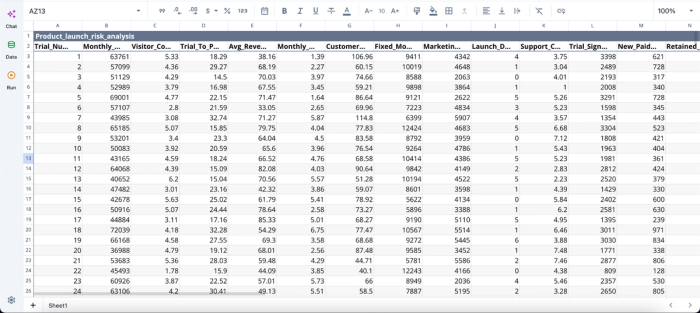
After importing our dataset into Quadratic, I can immediately begin analysis:
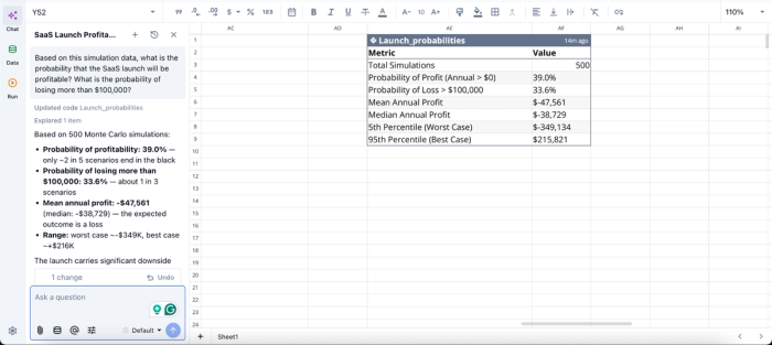
In this image, I ask Quadratic AI, “Based on this simulation data, what is the probability that the SaaS launch will be profitable? What is the probability of losing more than $100,000?” It instantly scans through the dataset and generates a table that gives insights into the probability of profit and loss, the projected mean annual profit, and other risk analysis-related metrics.
Share simulation models without breaking transparency
One of the persistent problems with spreadsheet-based simulations is that the underlying logic becomes difficult for reviewers to inspect. Complex formulas hide assumptions that require an Excel formula explainer, add-ins obscure mechanics, and workbook copies drift between users.
Quadratic keeps the assumptions in visible spreadsheet cells and the simulation logic in readable Python blocks directly inside the same file. Since it’s a collaborative analytics platform with real-time collaboration, multiple stakeholders can inspect and interact with the same live model simultaneously.
A finance director reviewing assumptions can focus on the spreadsheet layer while a quantitative analyst validates the Python simulation code underneath. Both perspectives exist inside the same collaborative environment.
Visualizations in Quadratic can also be done using text prompts. Here:
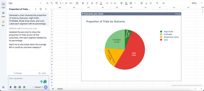
In this image, I ask Quadratic AI to “Generate a chart showing the proportion of trials by Outcome: High Profit, Profitable, Break-Even Zone, and Loss. Label each segment with its percentage.” In seconds, it creates a pie chart that shows the proportion of trials by outcome.
Conclusion: stop fighting the grid you have
The friction analysts feel when running Monte Carlo simulation Excel workflows comes from four specific places. They include volatile RAND that reshuffles results on every edit, Data Tables stretched into iteration engines they were never meant to be, the absence of seeding that makes runs irreproducible, and manual charting that disconnects outputs from the simulation that produced them. None of those are skill issues. They are structural properties of the tool.
The fix is to move the simulation engine to something built for iteration while keeping the spreadsheet interface that makes models legible to the people reviewing them.
Quadratic allows you to build your Monte Carlo model with a spreadsheet structure, Python-powered simulation, and charts in one file. The next time you open the workbook, the run you saved will be the run you see, and the friction you used to associate with the Monte Carlo simulation in Excel will simply not be there. Try Quadratic for free.
Frequently asked questions (FAQs)
What is the main problem with running a Monte Carlo simulation in Excel?
Excel's volatile RAND function recalculates on every edit, save, and keystroke, which means your simulation results change unpredictably and cannot be reliably reproduced. Combined with the misuse of Data Tables as iteration engines and disconnected charting, Excel creates friction at every stage of a Monte Carlo simulation workflow. These are structural limitations of the tool, not skill gaps on the analyst's part.
How does Quadratic address the limitations of Monte Carlo simulation in Excel?
Quadratic runs native Python directly in the same spreadsheet grid as your assumptions and formulas, giving you access to numpy.random and scipy.stats libraries. This means you can set an explicit seed so the same inputs always produce the same distribution and render histograms and convergence plots inline as the simulation runs. Your assumptions stay visible in cells where reviewers expect them, while the simulation logic lives in readable Python code blocks alongside the outputs it produces.
What does reproducibility mean in the context of Monte Carlo simulation?
Reproducibility means that the same random seed combined with the same assumptions always produces the same distribution of outcomes. This is essential for financial modeling and external audits, where you need to tie a specific result back to a specific run. Excel's RAND function cannot guarantee this because it has no seeding mechanism, making it impossible to defend or audit a simulation after the fact.